Introduction
This material covers key points of BBU6504: Data Mining.
Note
Some parts of material are adapted from the BBU6504 lecture slides and is intended for personal study and educational use only.
Lecture1: Introuction
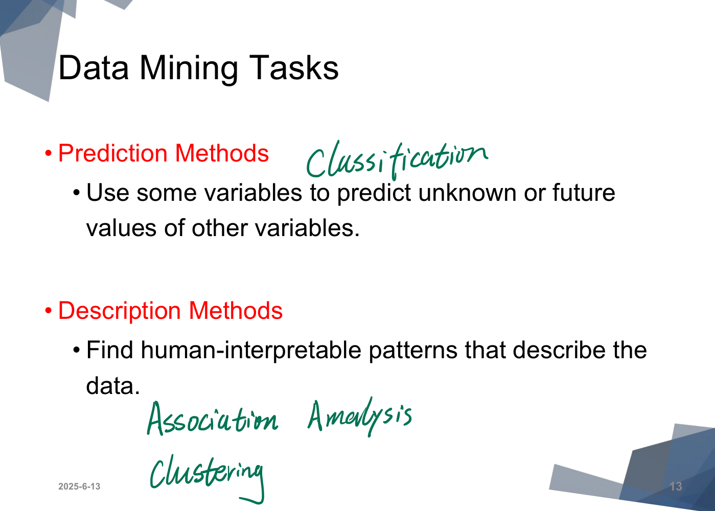
What is Data Mining?
KDD - Knowledge discovery in database
-
GET unknown and potentially useful information from data
-
Exploration & analysis, by automatic or semi-automatic means, of large quantities of data in order to discover
Attribute
| Type | Ordered | Differences Meaningful | True Zero | Ratios Valid |
|---|---|---|---|---|
| Nominal | No | No | No | No |
| Ordinal | Yes | No | No | No |
| Interval | Yes | Yes | No | No |
| Ratio | Yes | Yes | Yes | Yes |
Noise
For objects, noise is an extraneous object For attributes, noise refers to modification of original values
Outliers
Outliers are data objects with characteristics that are considerably different than most of the other data objects in the data set.
- Case 1: Outliers are noise that interferes with data analysis
- Case 2: Outliers are the goal of our analysis
Duplicate Data
Duplicate data refers to records that are exactly or nearly identical.
Cause: It’s common when merging datasets from heterogeneous sources.
Example:
- Same person appearing multiple times with different height values.
How to Handle:
- Remove exact duplicates.
- Merge similar records.
- Resolve conflicting values (e.g., take average or most recent).
Data cleaning: Process of dealing with duplicate data issues
When Not to Remove:
- When duplicates represent real events (e.g., Transactional context).
- When frequency matters (e.g., in pattern mining).
Lecture2 Quality, Preprocessing, and Measures
Preprocessing
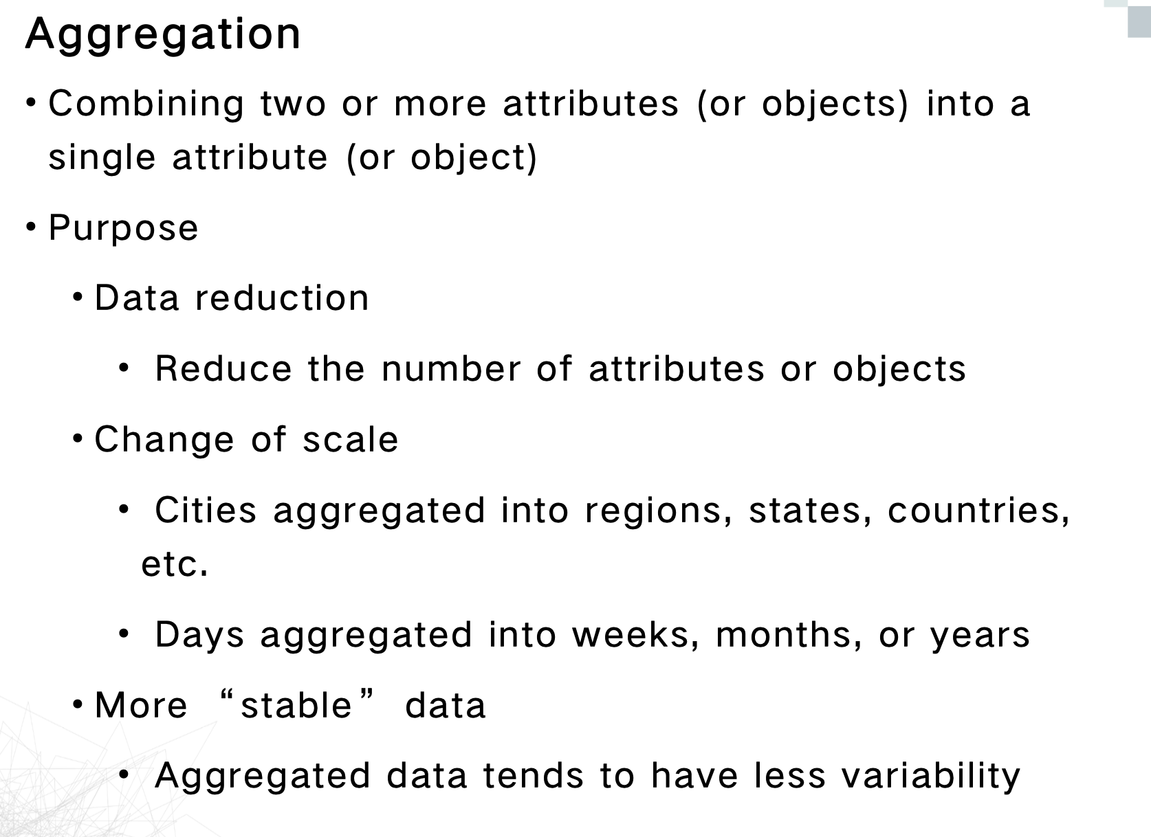
Aggregation
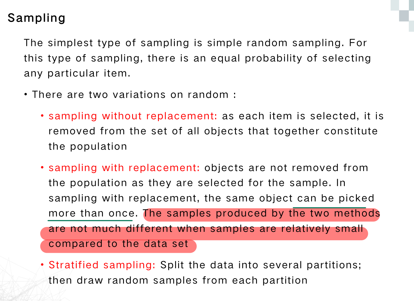
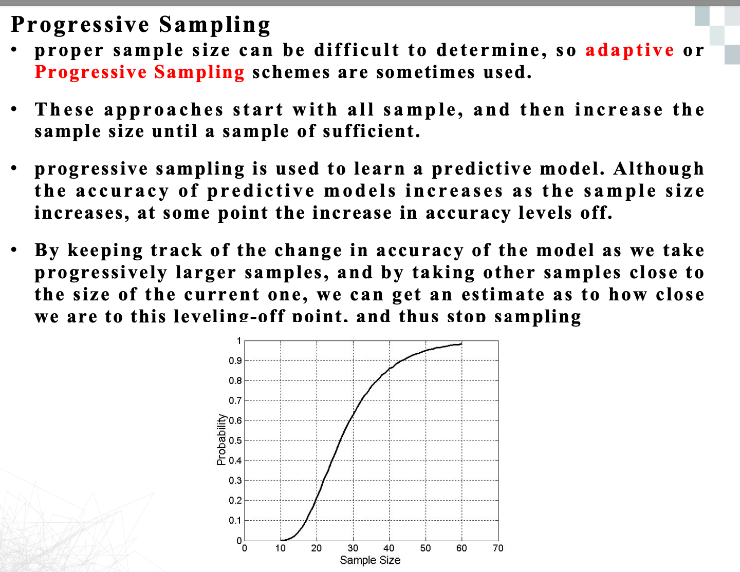
Sampling
Curse of Dimensionality
1.数据变稀疏
高维空间里,大多数数据点之间的距离都变得“差不多远”,密度差异变得不明显,这会导致很多算法(特别是依赖“距离”的算法,比如KNN、聚类)难以判断哪些点是“相近”的。
2.样本不够代表性
在高维空间中,可能需要指数级更多的样本才能覆盖整个空间。我们手头的数据,很可能根本不具代表性,训练出的模型泛化能力差。
3.分类器效果变差
对于分类任务,维度太高可能导致:
- 模型难以覆盖所有可能的“输入组合”
- 训练数据不足,模型容易过拟合
4.聚类质量下降
聚类依赖于“点与点之间的距离”来划分簇,但在高维中距离变得没意义,导致聚类结构模糊,效果差。
1. Dimensionality Reduction
Goal: Transform data into a lower-dimensional space while preserving as much useful information as possible.
Benefits:
- Avoids the curse of dimensionality
- Reduces time and memory consumption
- Makes data easier to visualize
- Helps remove noise and irrelevant patterns
Techniques:
- PCA (Principal Component Analysis): Projects data into components that capture the most variance
- SVD (Singular Value Decomposition): Matrix factorization to extract latent structure
- Other methods: t-SNE, autoencoders, LDA (depending on the task)
2. Feature Subset Selection
Goal: Select a subset of the most relevant features instead of transforming them.
Types of Features to Remove:
- Redundant features: Overlap with others in information (e.g., price and sales tax)
- Irrelevant features: Unrelated to the task (e.g., student ID when predicting GPA)
Benefits:
- Improves model performance and interpretability
- Speeds up training
- Reduces risk of overfitting
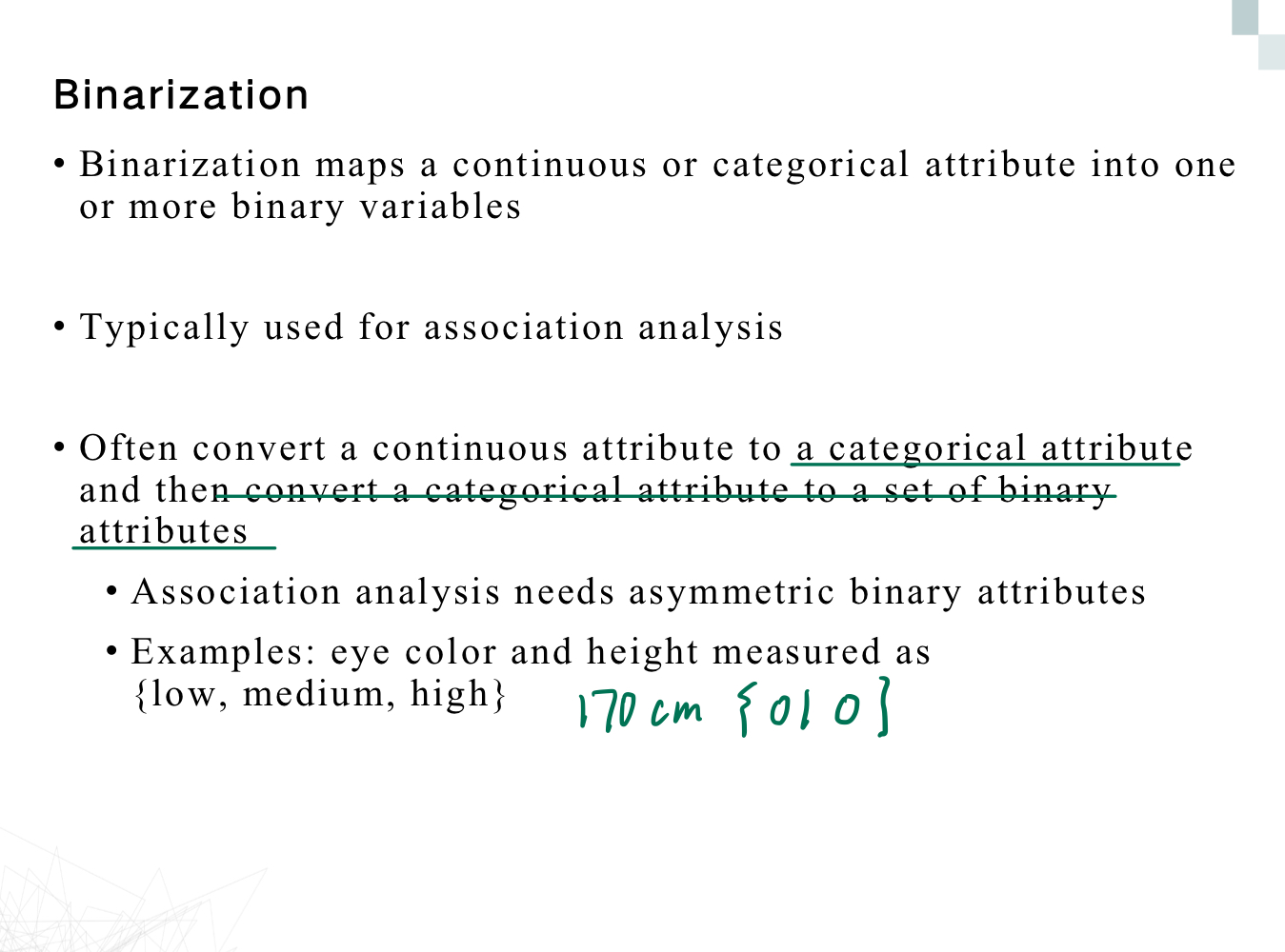
Binarization
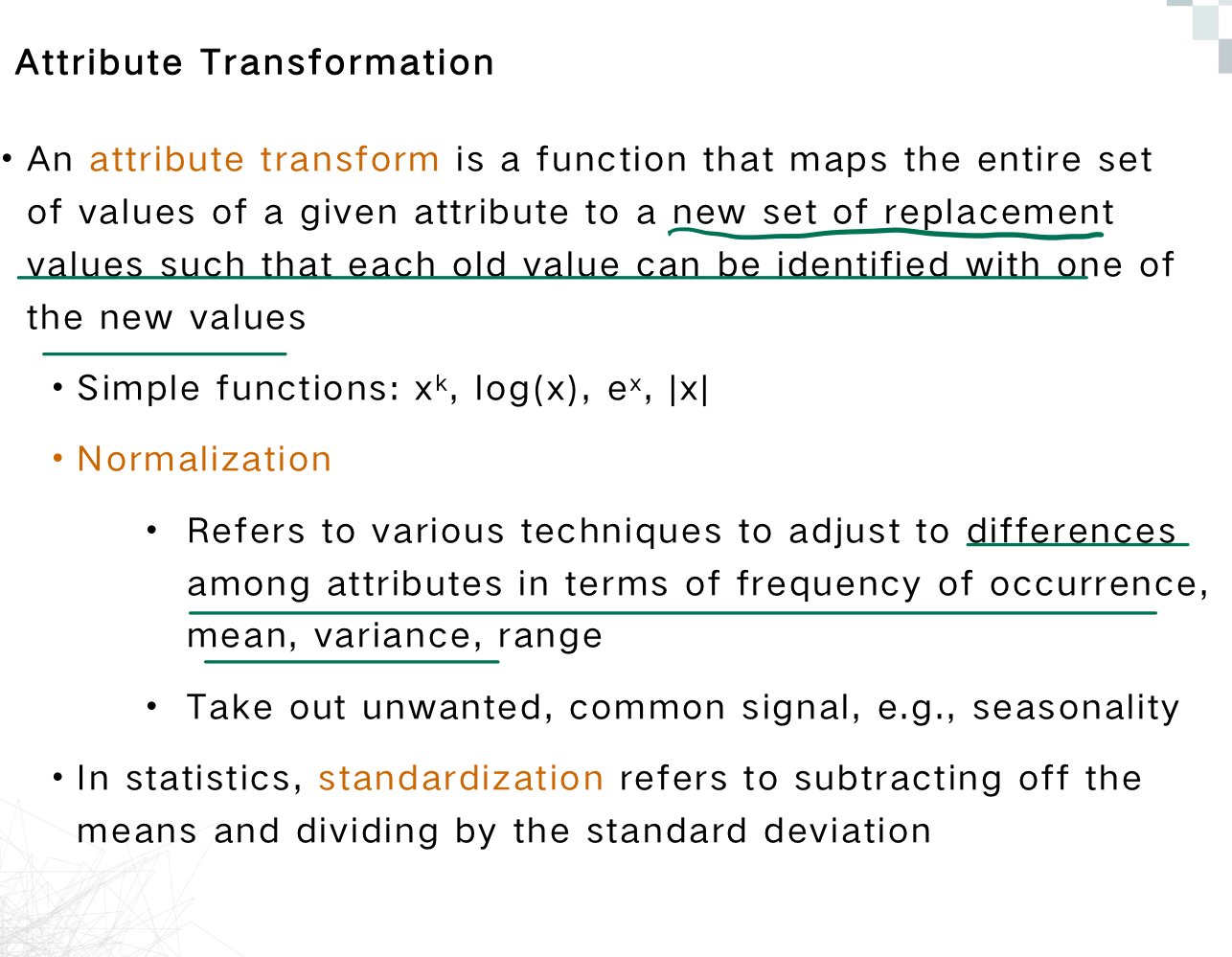
Attribute Transformation
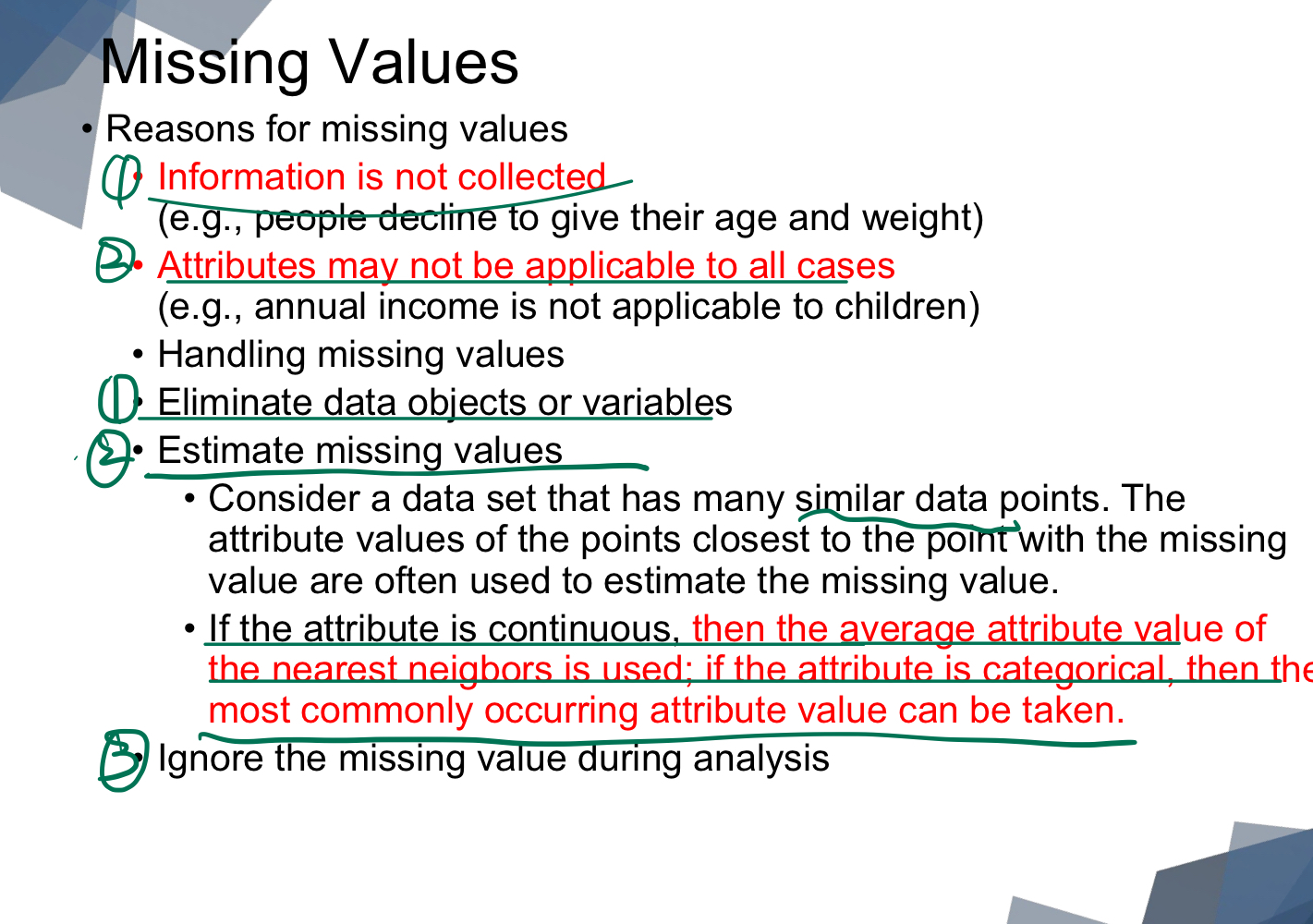
Missing Values
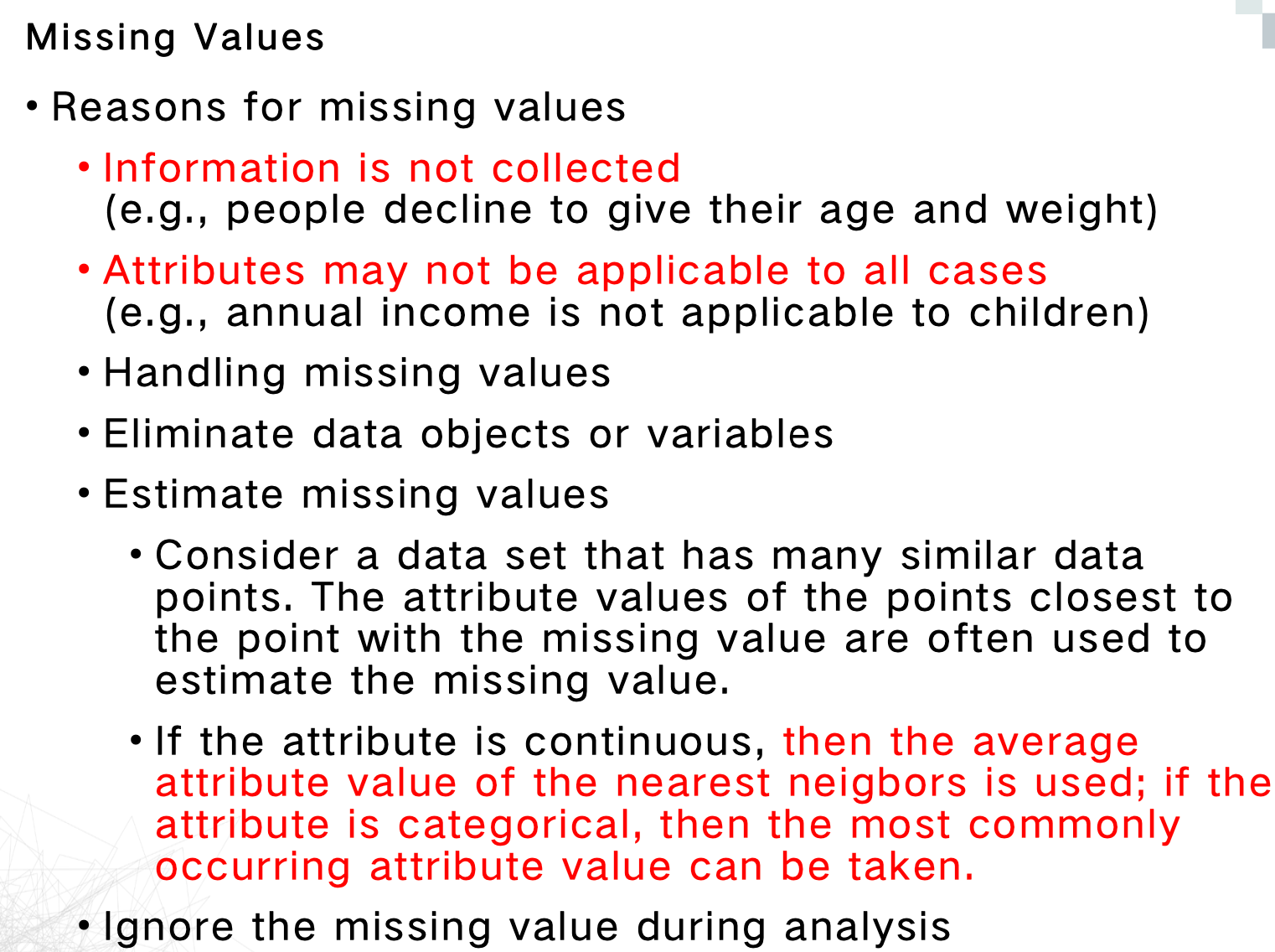
| Continuous | Use mean, median, or average of nearest neighbors |
|---|---|
| Categorical | Use mode, most frequent among nearest neighbors |
Similarity Measures
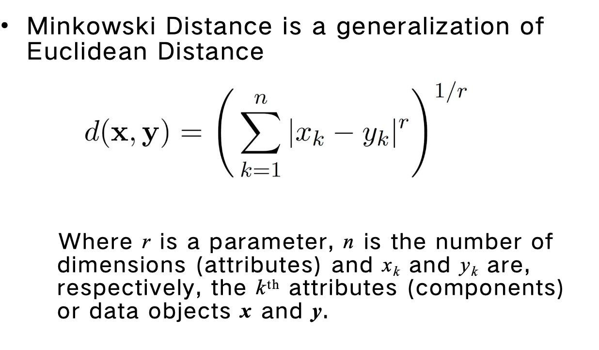
Minkowski Distance
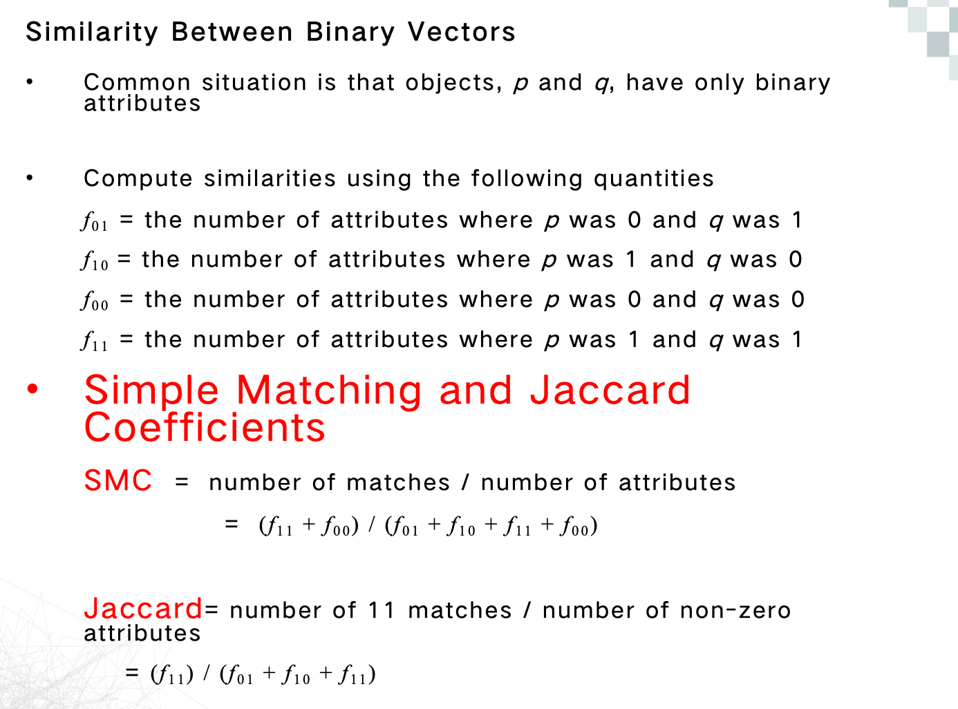
SMC and Jaccard
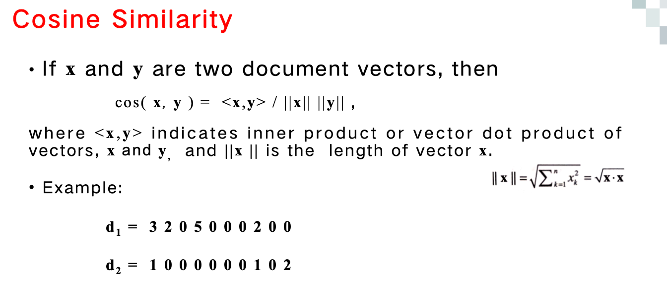
Cosine Similarity
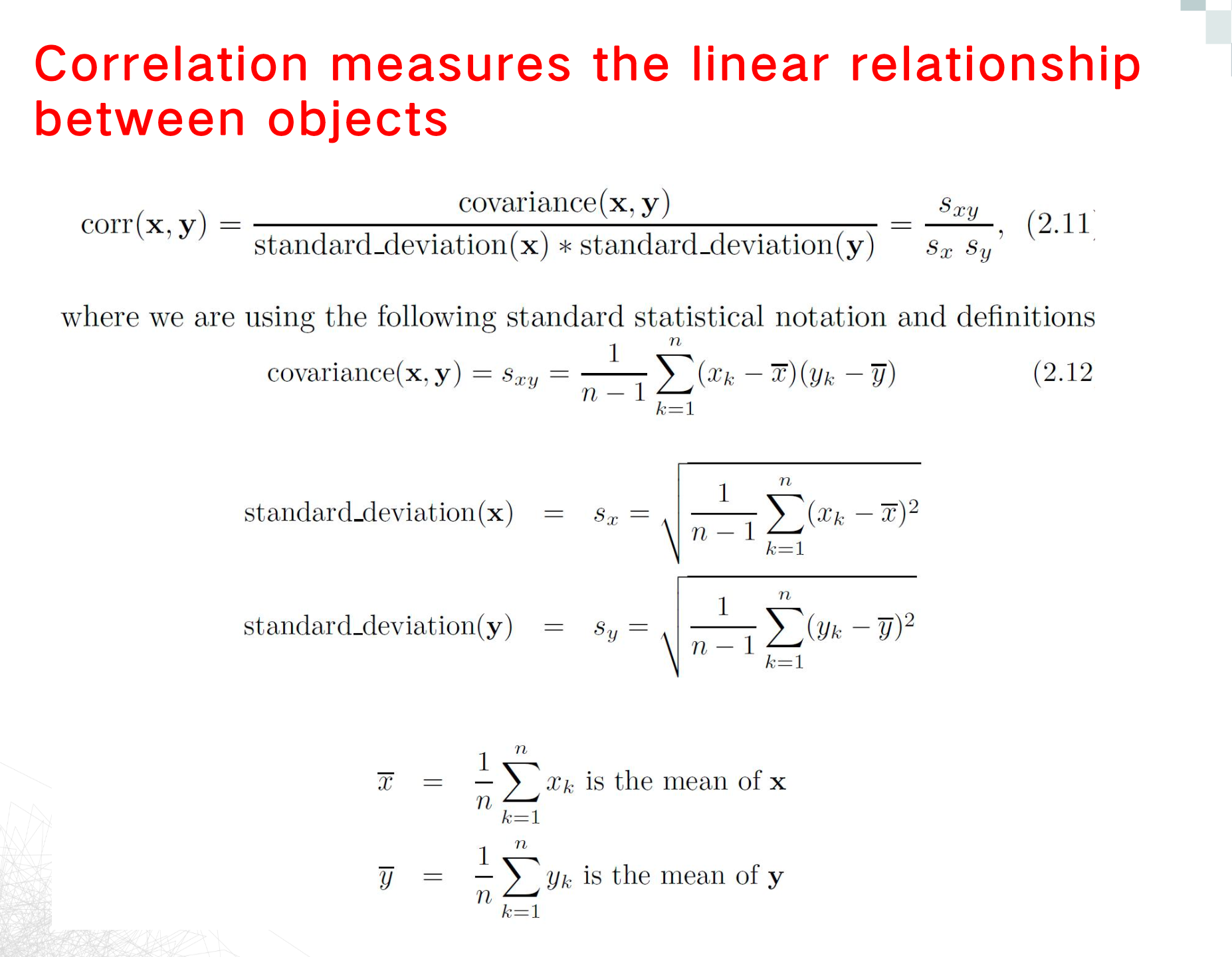
Correlation
| 方法 | 类型 | 适用数据 | 关注重点 | 推荐场景 | 不适合 |
|---|---|---|---|---|---|
| Euclidean Distance欧几里得距离 | 距离 | 数值型(连续) | 值的大小差异 | 聚类(如K-means)、低维连续数据 | 不适合高维稀疏数据 |
| Cosine Similarity余弦相似度 | 相似度 | 数值型(稀疏向量) | 方向/比例结构(忽略大小) | 文本向量、用户兴趣、TF-IDF | 不适合需要关注绝对大小的任务 |
| Correlation相关系数 | 相似度 | 数值型 | 变量间变化趋势(线性关系) | 时间序列趋势比较、评分模式对比 | 忽略绝对值,不适合关注“量”的场景 |
| SMCSimple Matching Coefficient | 相似度 | 二值型(对称) | 0 和 1 匹配都重要 | 投票、性别、偏好 | 不适合稀疏的行为数据(多数是0) |
| Jaccard Similarity | 相似度 | 二值型(非对称) | 1 的共现匹配,忽略 0 | 医疗记录、用户行为、标签数据 | 特征密集时不敏感,不能用于对称0-1 |
Clustering
- Well-separated
- Prototype-based
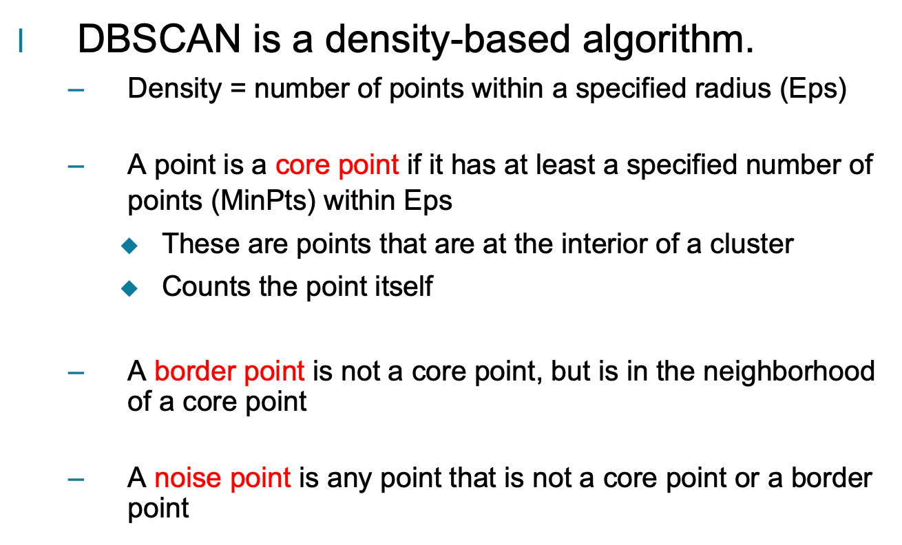
- Density-based
OR
- Hierarchical
- Partitional
- Density-based
K-means
K-means has problems when clusters are of differing Sizes,Densities
Non-globular shapes
K-means has problems when the data contains outliers.
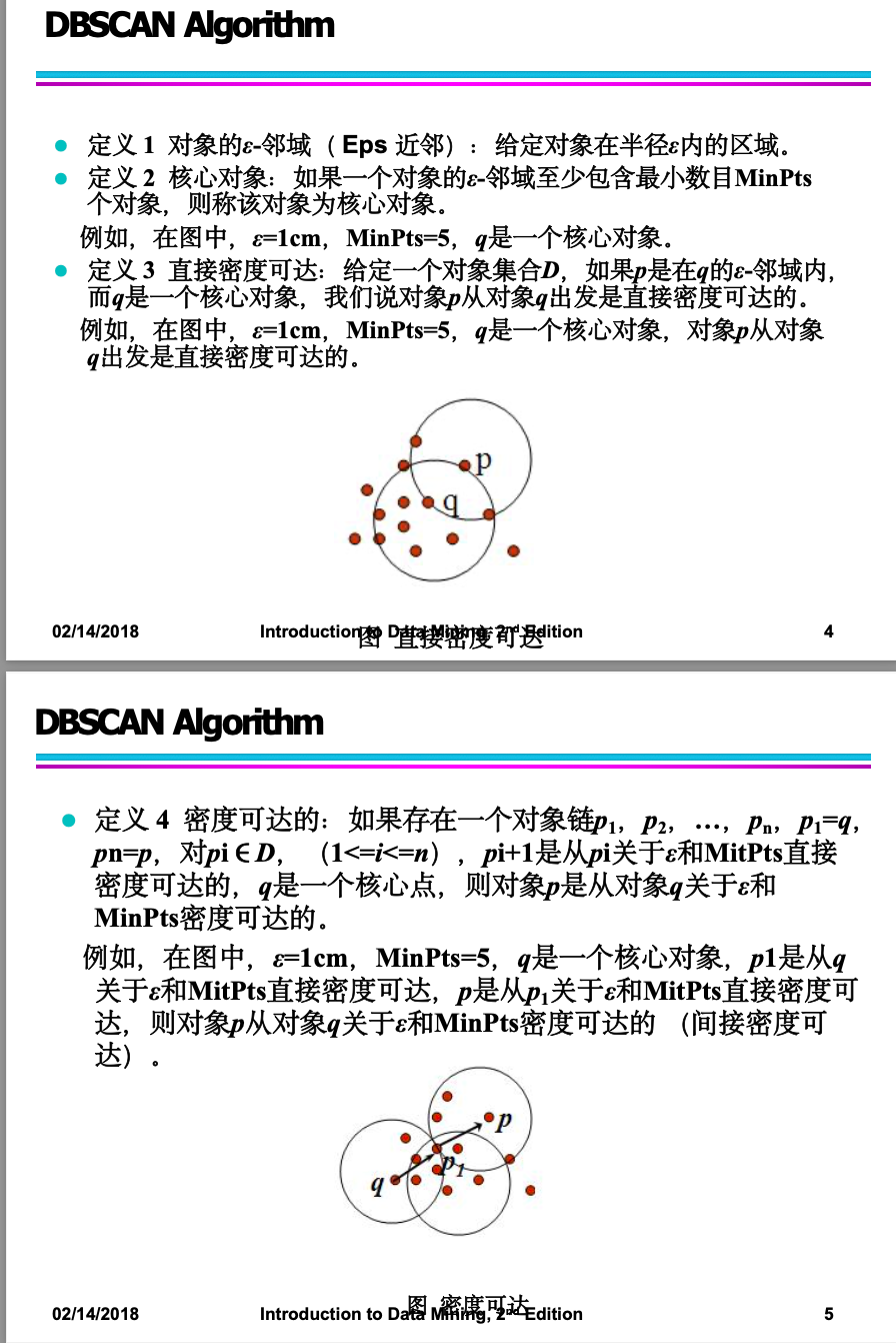
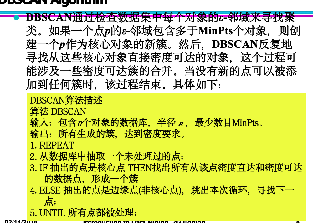
DBSCAN
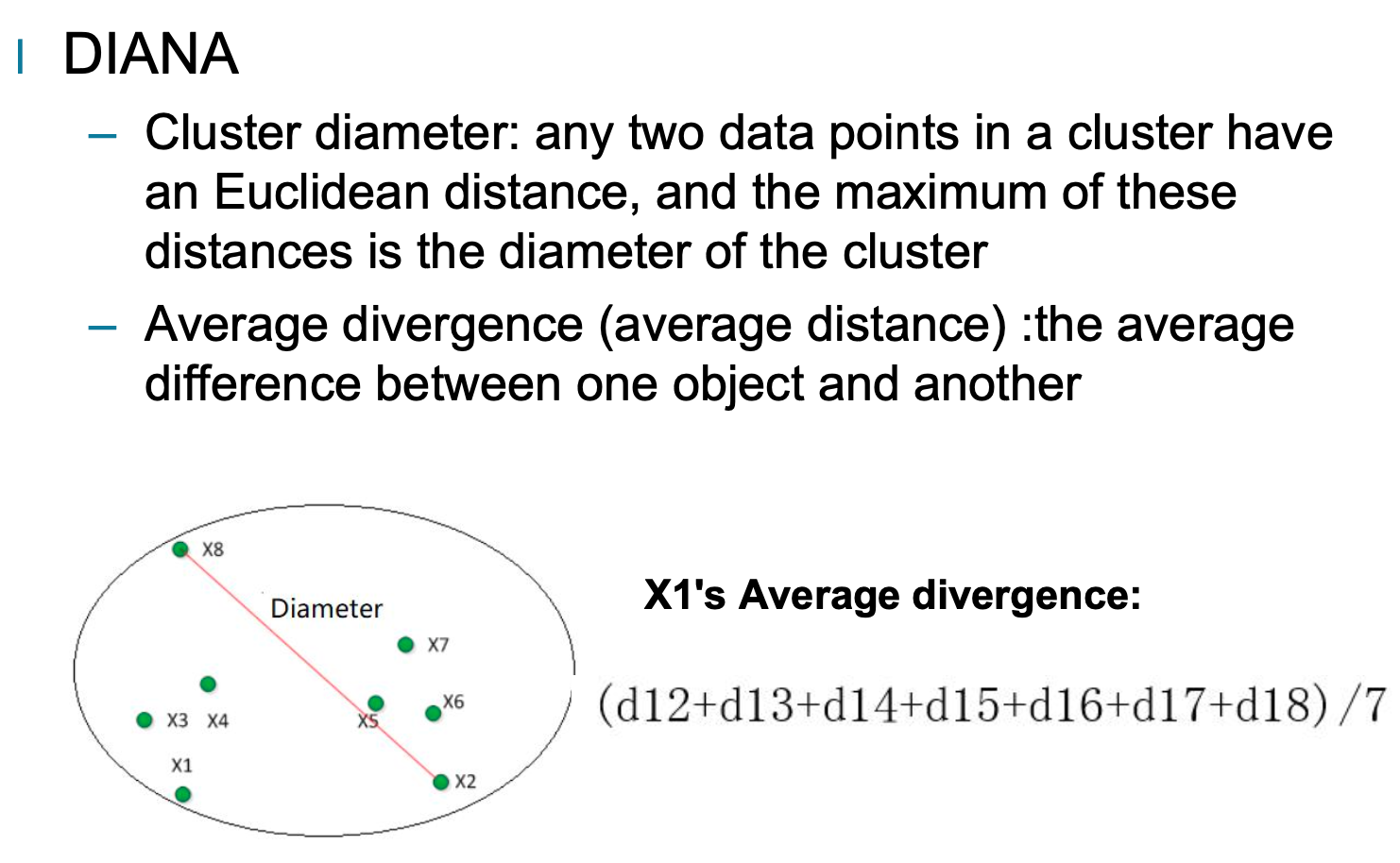
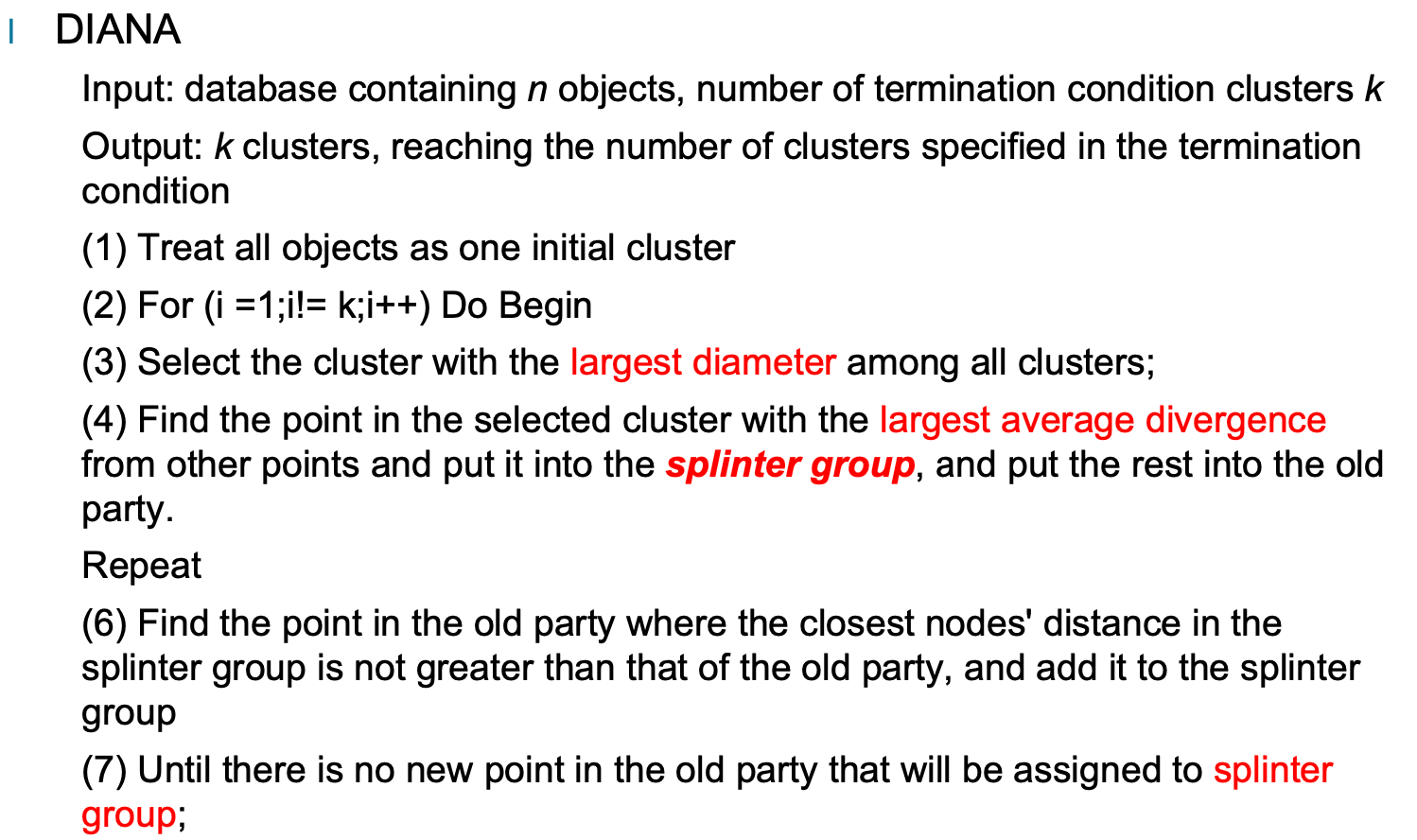
Diana
Agglomerative Hierarchical Clustering
Advantages and Disadvantages of Linkage
1. MIN (Single Linkage)
Advantages:
- Can handle clusters with non-elliptical shapes (e.g., elongated or curved).
- Simple to compute, only considers the shortest distance between clusters.
Disadvantages:
- Prone to the chaining effect, where loosely related points form long chains.
- Highly sensitive to noise and outliers, which can act as bridges between clusters.
2. MAX (Complete Linkage)
Advantages:
- More robust to noise and outliers, as it uses the farthest points to determine proximity.
- Tends to produce compact and well-separated clusters.
Disadvantages:
- May fail to merge naturally connected but irregularly shaped clusters.
- Sensitive to cluster density differences; sparse clusters may be split unnecessarily.
3. Group Average Linkage
Advantages:
- Balances between Single and Complete Link methods.
- Less sensitive to noise and avoids chaining effect.
- Can handle complex and non-spherical cluster shapes effectively.
Disadvantages:
- Higher computational cost due to averaging all point pairs between clusters.
- Sensitive to differences in cluster size and density, which may distort proximity values.
Problems and Limitations
-
Once a decision is made to combine two clusters, it cannot be undone
-
No global objective function is directly minimized
-
Different schemes have problems with one or more of the following:
– Sensitivity to noise and outliers
– If the splitting point is not selected at a certain step, it may result in low-quality clustering results.
– Big data sets don’t break very well.
Q: How to overcome the limitation that “movement is the ultimate” in hierarchical clustering?
This limitation means that once two clusters are merged, the decision cannot be undone. To overcome this:
-
Post-processing by moving branches in the dendrogram:
After constructing the initial hierarchy, the structure of the dendrogram can be refined by moving subtrees (branches) to new positions to better optimize a global objective function (e.g., minimizing overall variance or improving silhouette score). This allows corrections to be made to earlier poor merging decisions.
-
Hybrid approach using partitional clustering first:
Another method is to first use a partitional algorithm like K-means to divide the data into many small, dense clusters. Then, hierarchical clustering is applied to these clusters instead of individual data points. This reduces the impact of noise and prevents early incorrect merges, leading to a more robust hierarchy.
Advanced Cluster Analysis
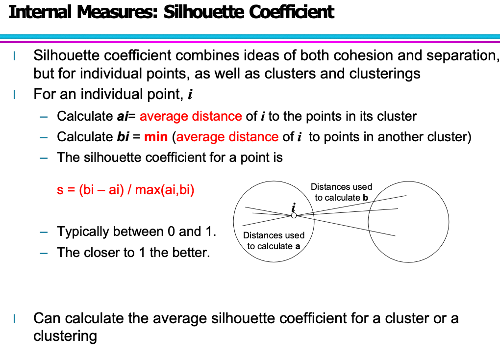
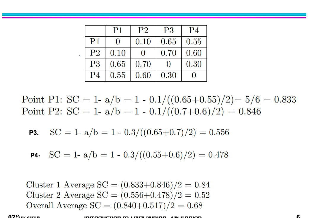
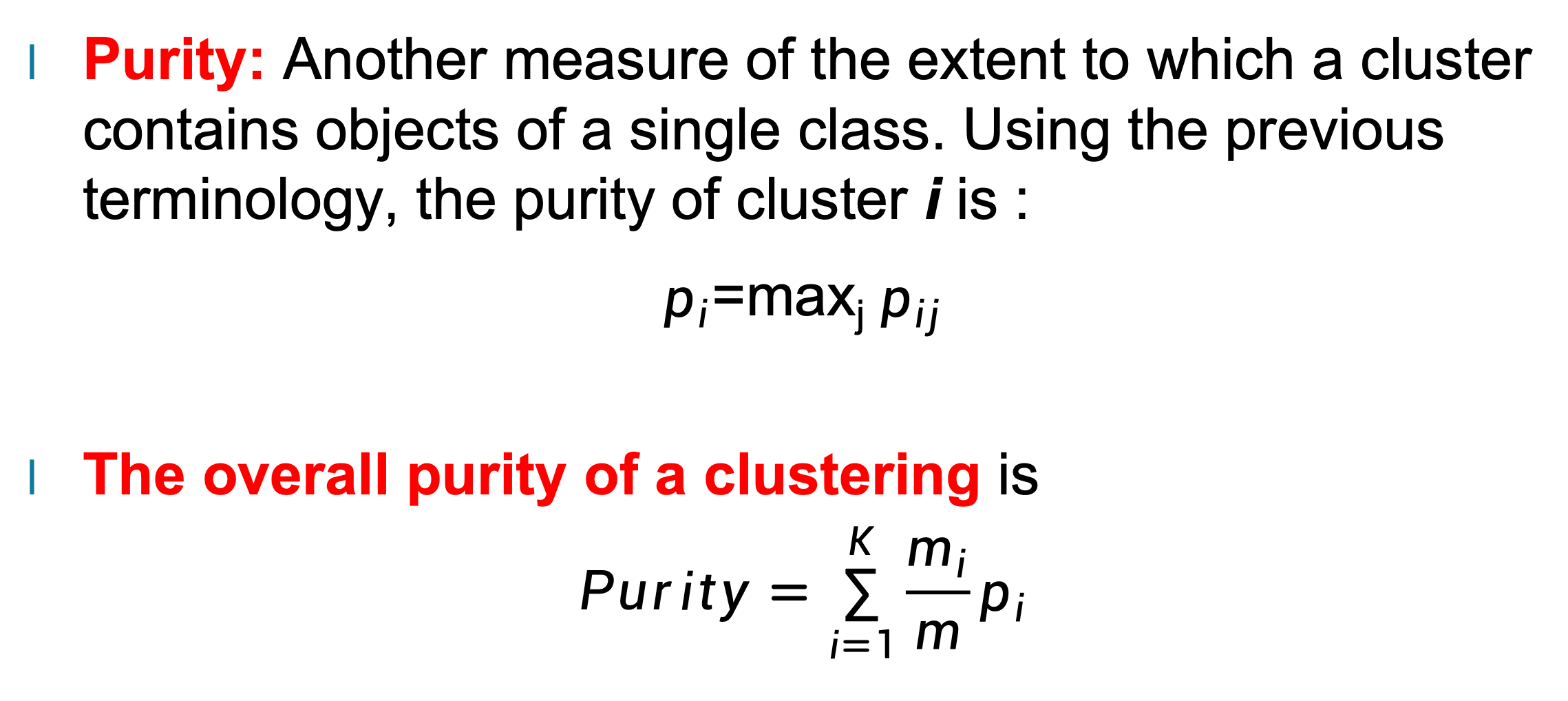
Silhouette
Cluster 1 contains {P1, P2}, Cluster 2 contains {P3, P4}. The dissimilarity matrix that we obtain from the similarity matrix is the following:
Decision Tree
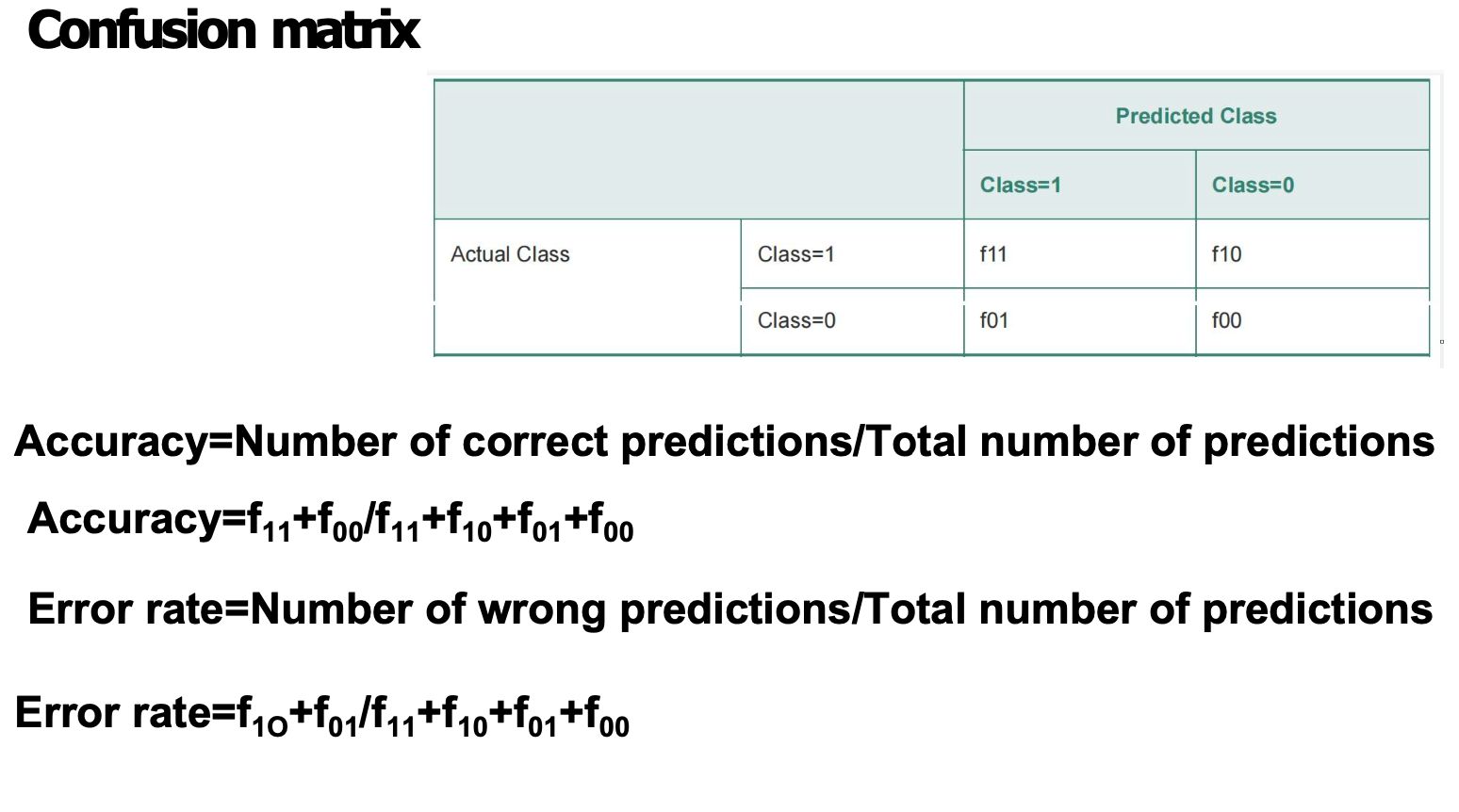
Confusion Matrix
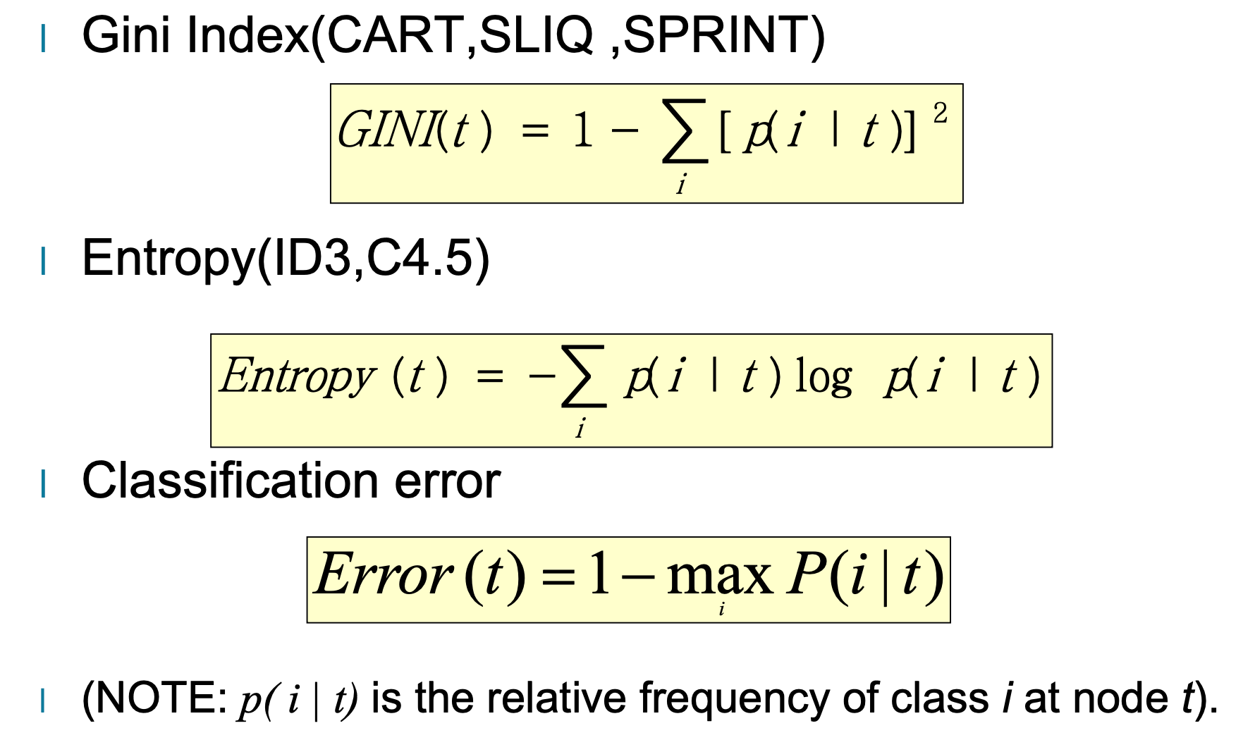
Impurity Calculation ( Will be asessed)
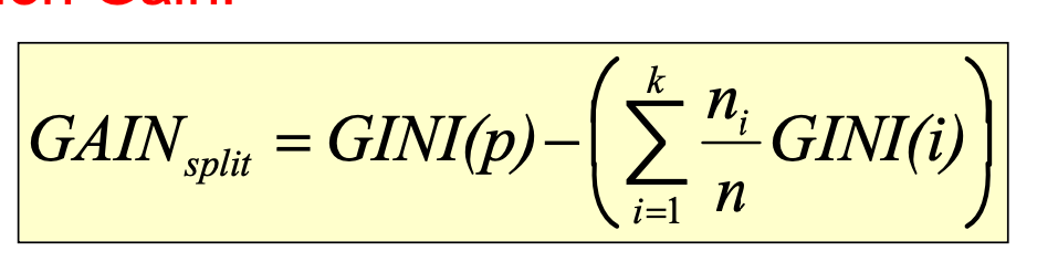
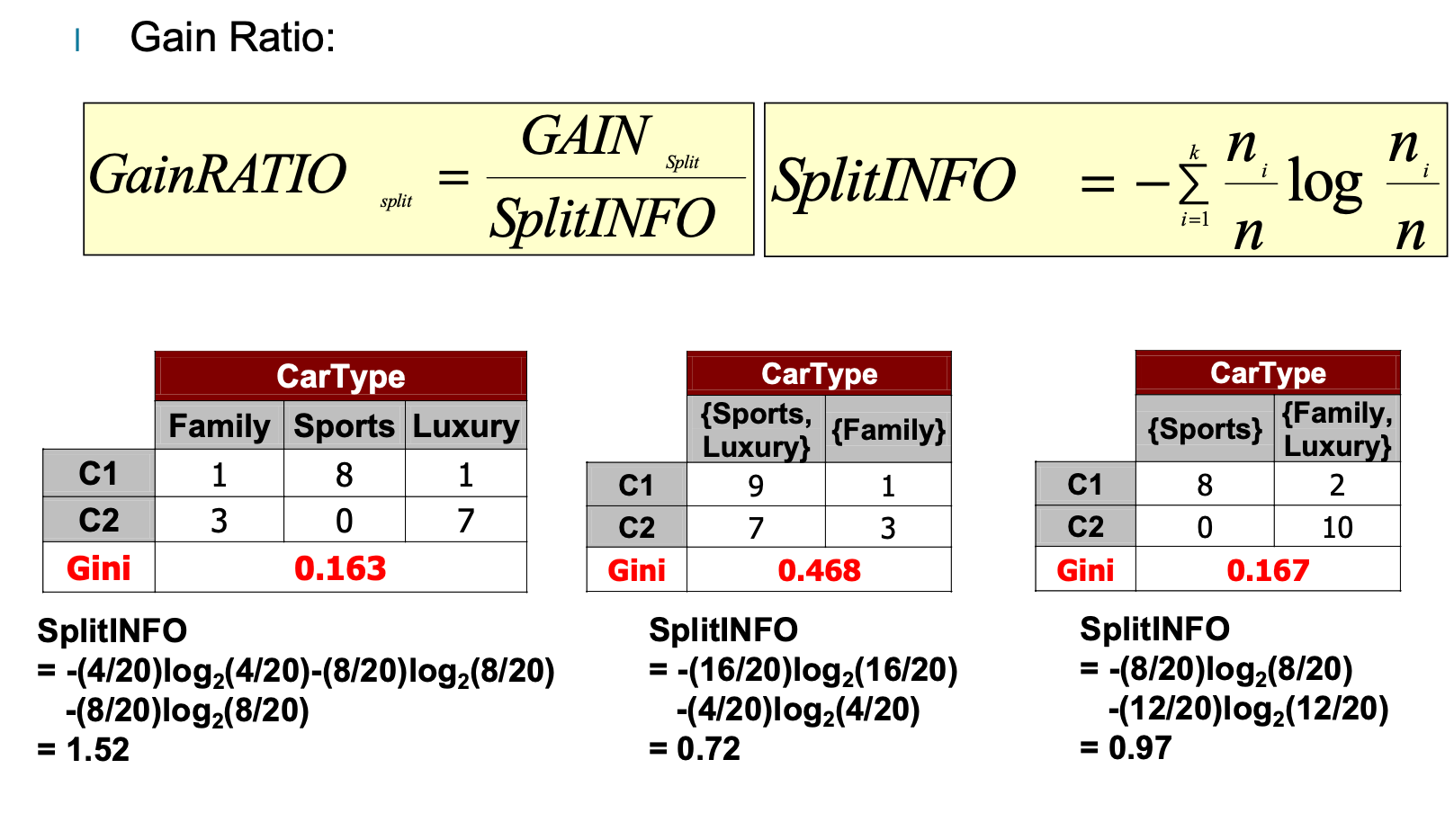
Gini gain
Gain ratio
Node impurity measures tend to prefer splits that result in large number of partitions, each being small but pure.
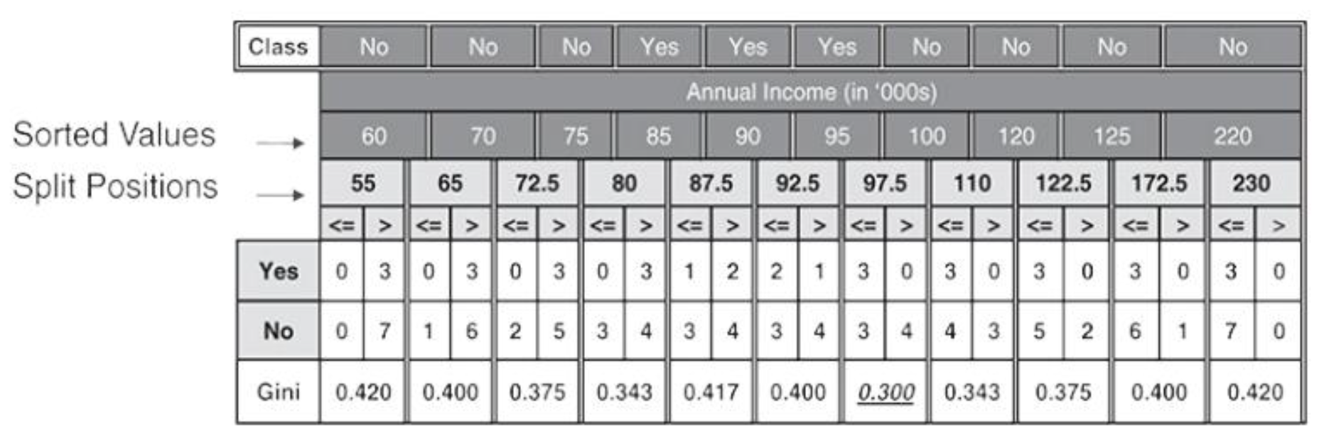
Finding The Best Split for Continuous Attributes
For efficient computation o(nlogn) compared to brute-force(N^2):
- – Sort the attribute based on their values
- – Calculate the midpoints between two adjacent sorted values
- – Linearly scan these midpoints, each time updating the count matrix and computing Gini index
- – Choose the split position that has the least Gini index
Pros & Cons
Advantages:
- – Inexpensive to construct
- – Extremely fast at classifying unknown records
- – Easy to interpret for small-sized trees
- – Robust to noise(especially when methods to avoid overfitting are employed)
- – Can easily handle redundant or irrelevant attributes(unless the attributes are interacting)
Disadvantages:
- – Space of possible decision trees is exponentially large. Greedy approaches are often unable to find the best tree.NP-hard.
- – Handling Redundant Attributes:An attribute is redundantif it is strongly correlated with another attribute in the data. Since redundant attributes show similar gains in purity if they are selected for splitting, only one of them will be selected as an attribute test condition in the decision tree algorithm. Decision trees can thus handle the presence of redundant attributes.
- – Using Rectilinear Splits:The test conditions described so far in this chapter involve using only a single attribute at a time.
Q: Why would we choose Naive Bayes instead of decision trees in some scenarios?
In certain scenarios, Naive Bayes is preferred over decision trees for the following reasons:
-
High-dimensional data: Naive Bayes performs well with high-dimensional data, such as text classification, where each word is a feature. It remains effective even with a small number of training examples.In contrast, decision trees are prone to overfitting in such cases.
-
Faster training and prediction: Naive Bayes is computationally efficient because it only requires calculating probabilities. Decision trees need to search for optimal splits, which is more time-consuming.
-
Better performance with independent features: If features are mostly conditionally independent, Naive Bayes can be highly accurate. Decision trees may overfit when feature interactions are weak or noisy.
-
Robust to noise and missing data: Naive Bayes handles noisy and missing data gracefully, while decision trees can be sensitive and may produce overly complex models.
-
Small dataset:
Naive Bayes requires less data to estimate parameters, making it more suitable when training data is limited. Decision trees often need more data to build stable and generalizable models.
-
Flexible decision boundaries:
Decision trees can only form rectilinear (axis-aligned) boundaries, limiting their ability to model complex or diagonal class separations. Naive Bayes, especially with Gaussian distributions, can create elliptical or non-linear decision boundaries.
Classification-Evaluation
Overfitting and Underfitting
What is overfitting and underfitting?
Optimistic and Pessimistic
- Optimistic: Training error → generalisation error
- pessimistic :
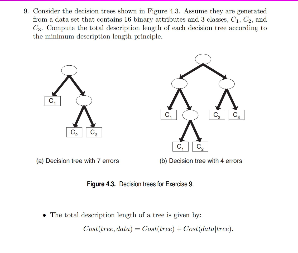
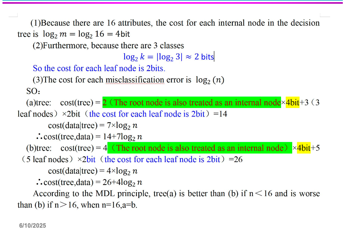
MDL
The model is encoded in compressed form before being passed to B. The cost of transmission is equal to the cost of model coding.
The total cost of transmission is:
$Cost(Model,Data) = Cost(Data|Model) + Cost(Model)$
Cost(Data|Model) :encodes the misclassification errors.
Cost(Model) :Model coding overhead
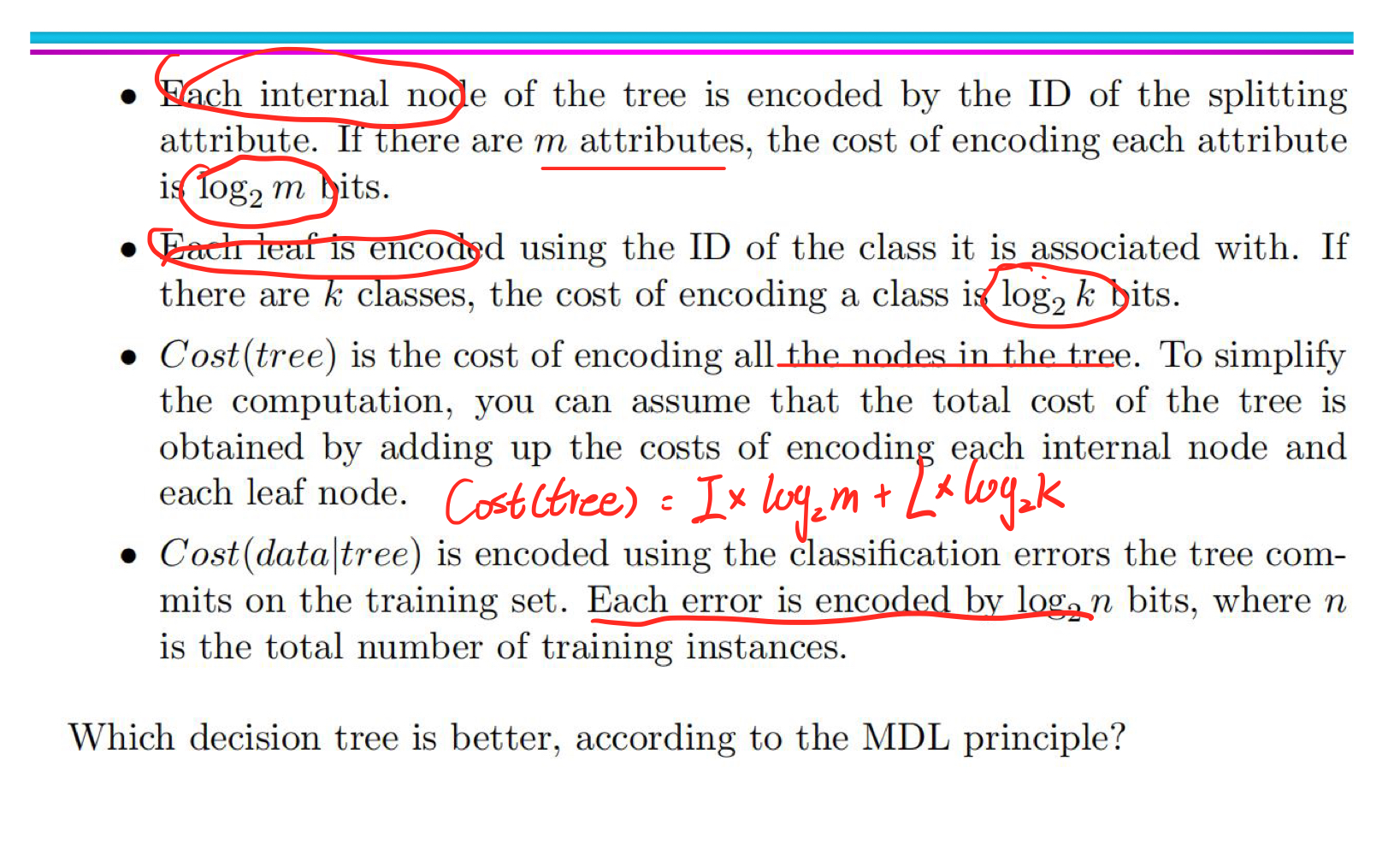
So the total cost should be:
$Cost(Model,Data)=N(Error) \times log_2n + N(Internal)\times log_2m + N(Leaf)\times Log_2k$
where n is the number of training instances, m is the number of attributes and k is the number of classes
Handling Overfiting
Pre-pruning
Stop the algorithm before it becomes a fully-grown tree
-
Stop if all instances belong to the same class
-
**Stop if all the attribute values are the same
More restrictive conditions:**
- Stop if number of instances is less than some user- specified threshold
- Stop if expanding the current node does not improve impurity measures (e.g., Gini or information gain).
- Stop if estimated generalization error falls below certain threshold
Pose-pruning
Subtree replacement
- If generalisation error improves after trimming, replace sub-tree by a leaf node
- Class label of leaf node is determined from majority class of instances in the sub-tree.
Subtree raising
- Replace subtree with most frequently used branch
Post-pruning tends to produce better results than pre-pruning, because unlike pre-pruning, post-pruning is a pruning decision based on a fully-growth decision tree. Pre-Pruning may terminate the growth of the decision tree too early. However, for post-pruning, when the subtree is cut off. The overhead of growing a complete decision tree is wasted
8.1 Alternative Classification Techniques
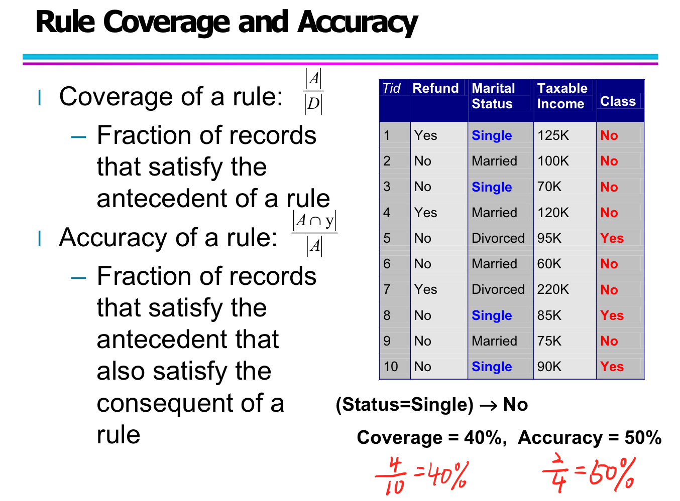
Rule-based Classifier
Rule coverage and accuracy
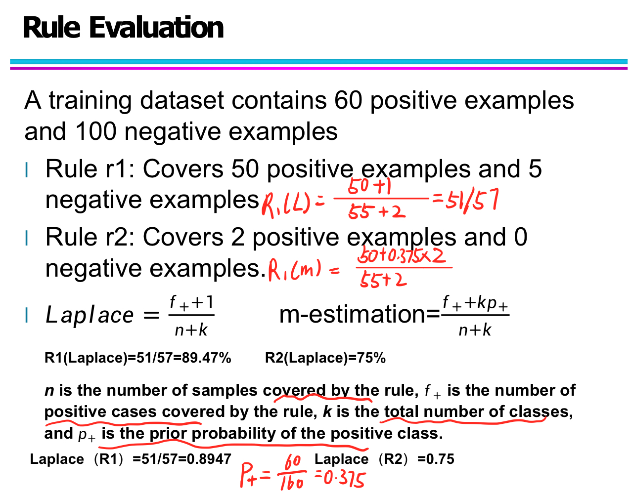
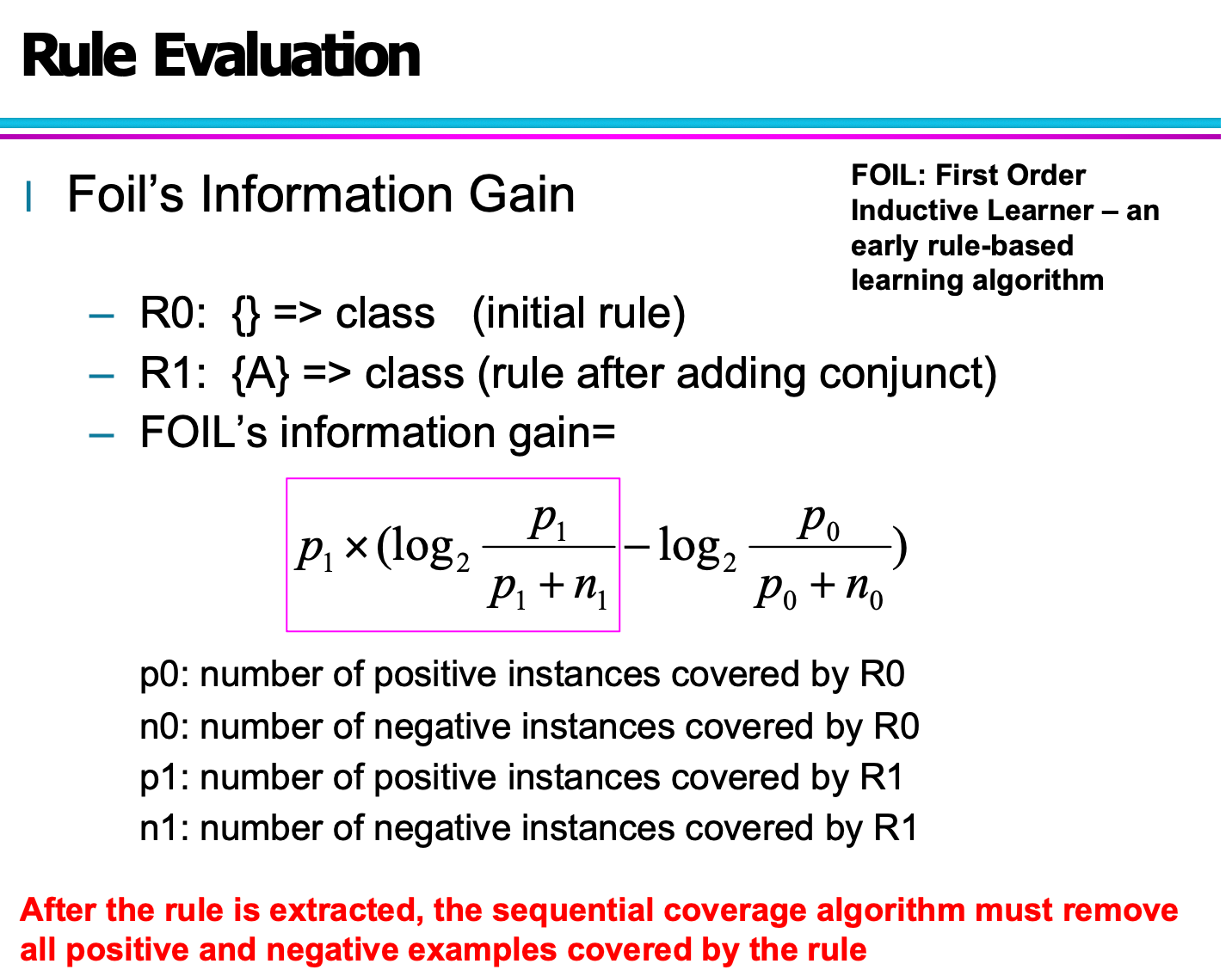
Rule Evaluation
Direct Method-RIPPER
RIPPER (Repeated Incremental Pruning to Produce Error Reduction) is a rule-based classification algorithm designed to efficiently generate a set of interpretable rules, especially for large datasets. It follows a direct rule-learning approach through sequential covering, pruning, and MDL-based stopping criteria.
Handling Class Labels
- Two-class problems:
- Choose the class with lower prevalence (fewer instances) as the positive class.
- The other becomes the default (negative) class, which is implicitly predicted when no rules match.
- Multi-class problems:
- Sort all classes in increasing order of prevalence.
- Learn rules for the smallest class first, treating all others as negative.
- Repeat the process for the next smallest class, and so on.
Growing a Rule
- Begin with an empty rule.
- Add conditions (conjuncts) incrementally to the rule as long as they increase FOIL’s information gain.
- Stop adding conditions when the rule starts covering negative examples.
- Prune the rule using a validation-based strategy:
-
Use the metric:
$$ v = \frac{p - n}{p + n} $$
where:
- p: number of positive instances covered in the validation set
- n: number of negative instances covered in the validation set
-
Remove any final sequence of conditions that maximizes v.
-
Building a Rule Set
- Use a sequential covering approach:
- Repeatedly find the best rule to cover the remaining positive examples.
- Remove all examples (both positive and negative) covered by the rule.
- After each rule is added, compute the total description length.
- Stop adding rules when the new rule set is d bits longer than the smallest description length found so far.
- Default threshold: d = 64
Indirect Method-C4.5
C4.5rules is an indirect rule-based classification method derived from the C4.5 decision tree algorithm. Instead of building rules directly from data, it extracts and simplifies rules from an unpruned decision tree, and then organizes them using the minimum description length (MDL) principle.
🔹 Rule Extraction and Simplification
-
Start by extracting rules from an unpruned decision tree.
-
Each rule takes the form:
A → y, where A is a conjunction of conditions (e.g., attribute tests), and y is a class label.
-
To simplify a rule, iteratively remove one condition (conjunct) to create a shorter version A′ → y.
-
For each simplified version:
- Compute the pessimistic error estimate.
- Retain the rule with the lowest pessimistic error, as long as its error is not worse than the original.
-
Repeat until no further improvement is possible.
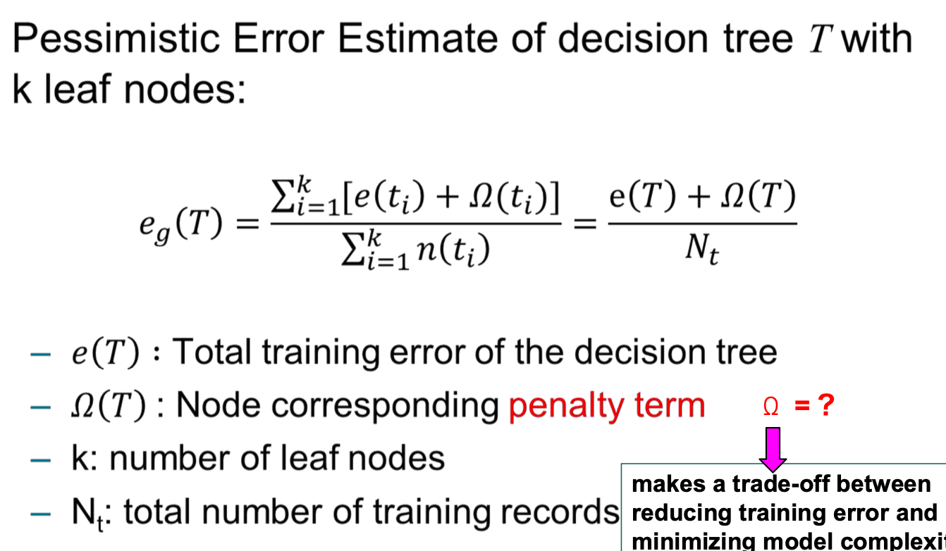
🔹 Pessimistic Error Estimate
To avoid overfitting, C4.5 uses a pessimistic estimate of a rule/tree’s error:
$e_g(T) = \frac{e(T) + l(T)}{N_t}$
Where:
- e(T): number of training errors in the tree
- l(T): penalty term (e.g., one per leaf node)
- $N_t$: total number of training samples
This formula penalizes complex models and favors generalization.
🔹 Class-Based Rule Set Organization
Instead of ordering rules linearly, C4.5rules orders subsets of rules grouped by class label. Each class has its own rule subset.
For each class subset:
- Compute its description length:
$\text{Description Length} = L(\text{error}) + g \cdot L(\text{model})$
Where:
- $L(\text{error})$: bits needed to encode misclassified examples
- $L(\text{model})$: bits needed to encode the rule model
- g: regularization parameter (default = 0.5), penalizes redundant attributes
Finally, order the classes by increasing total description length, prioritizing the most compact and accurate rule sets.
🔹 C4.5rules vs RIPPER – Rule Comparison Example
Given a dataset of animals with features like “Give Birth”, “Can Fly”, “Live in Water”, etc., both algorithms generate rule sets for classification.
C4.5rules:
- Extracted from decision tree paths
- Rule conditions follow attribute hierarchy
- Example rules:
- (Give Birth = No, Can Fly = Yes) → Birds
- (Give Birth = Yes) → Mammals
- (Give Birth = No, Can Fly = No, Live in Water = No) → Reptiles
RIPPER:
-
Grows rules directly from data using greedy heuristics (e.g., FOIL’s info gain)
-
Rules are more compact, with separate handling for default class
-
Example rules:
- (Live in Water = Yes) → Fishes
- (Have Legs = No) → Reptiles
- (Can Fly = Yes, Give Birth = No) → Birds
- Default → Mammals
Naive Baye
| Feature | C4.5rules | RIPPER |
|---|---|---|
| Method Type | Indirect (tree-based) | Direct (rule growing) |
| Rule Source | Decision tree paths | Data-driven search |
| Rule Simplification | Pessimistic error pruning | Post-pruning with FOIL gain |
| Class Handling | Class-based subsets (ordered by MDL) | Class-wise sequential covering |
| Default Class | Explicit rules | Implicit (default class at end) |
KNN (know)
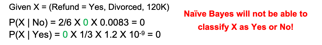
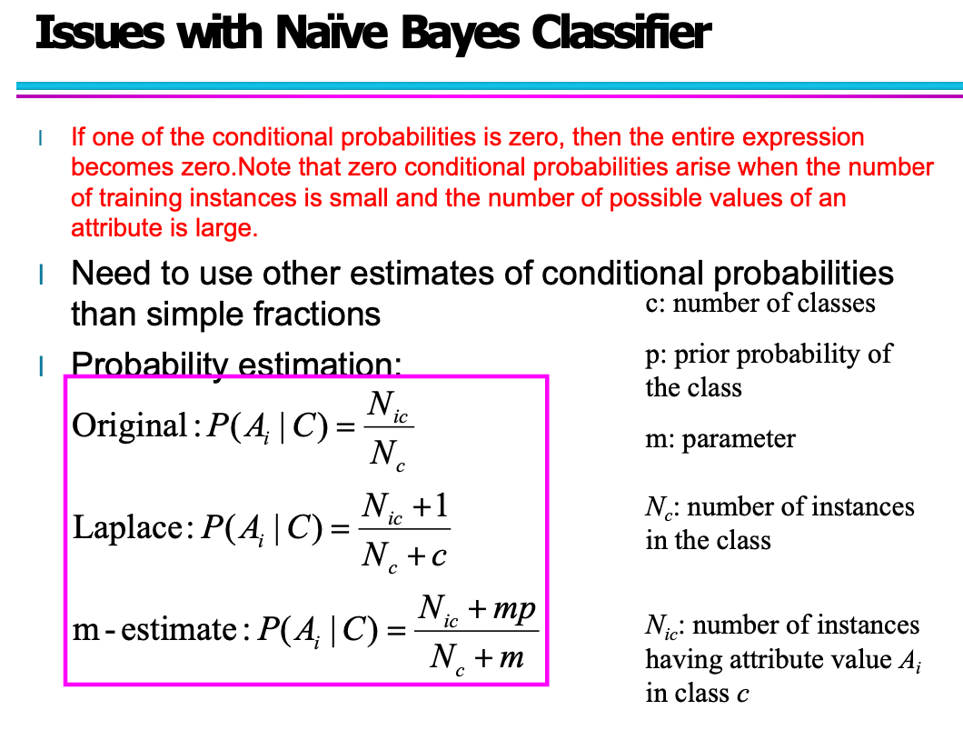
Bayes Classifier
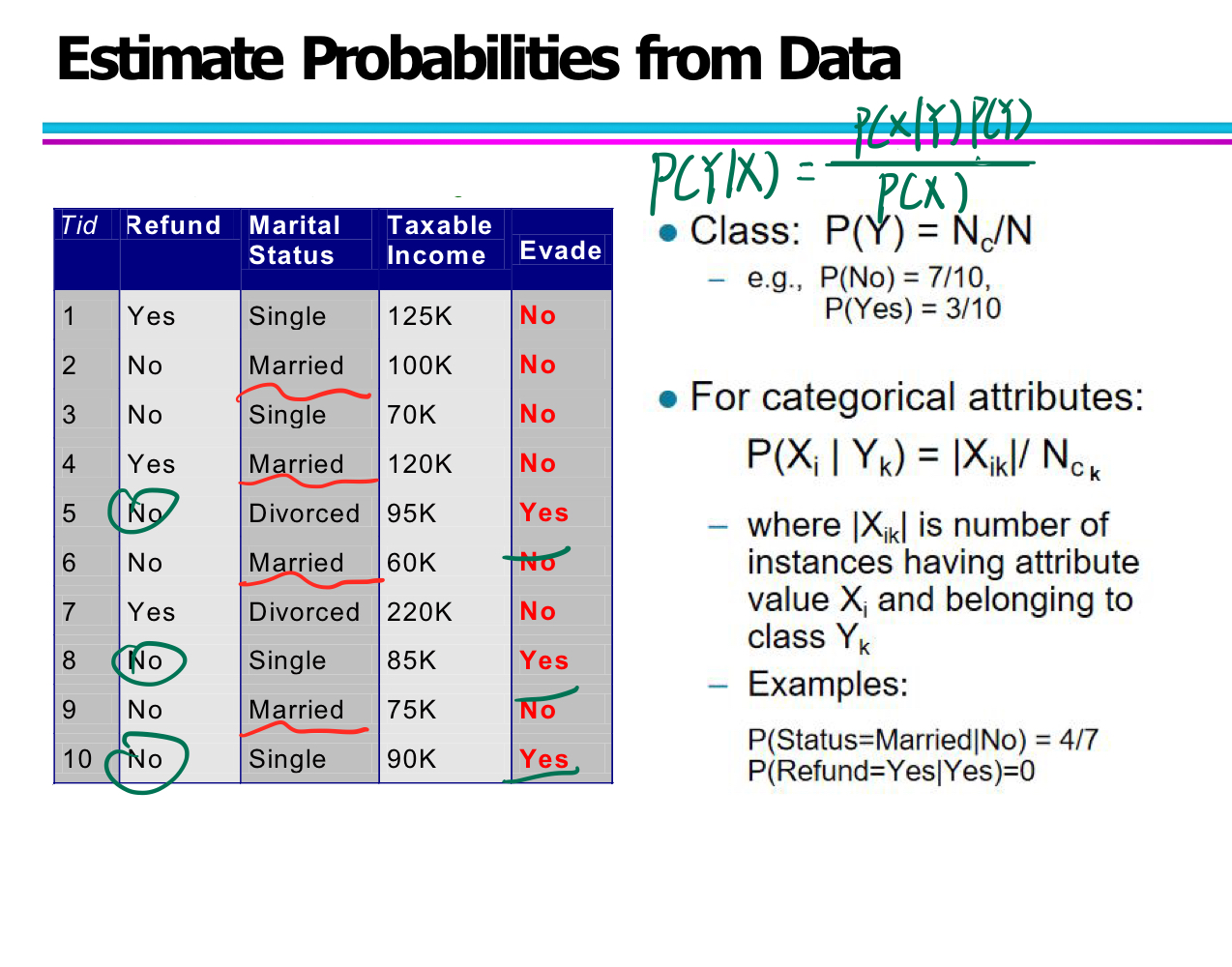
Estimate Probabilities from Data
In Naïve Bayes classification, we need to estimate the conditional probability of attributes given a class:
$P(X_i \mid Y_j)$
For continuous attributes, there are two main strategies:
1. Discretization
- Convert continuous attributes into categorical (ordinal) bins.
- Replace each value with its corresponding bin label.
- This changes the attribute from continuous to ordinal.
- Pros: simple to implement
- Cons: may lose precision and introduce arbitrary thresholds
2. Probability Density Estimation
- Assume that the attribute values follow a normal (Gaussian) distribution for each class.
- Estimate the mean (μ) and variance (σ²) for each attribute–class pair using the training data.
- Use the Gaussian probability density function to compute conditional probability:
$P(X_i = x \mid Y_j) = \frac{1}{\sqrt{2\pi \sigma_{ij}^2}} \cdot e^{-\frac{(x - \mu_{ij})^2}{2 \sigma_{ij}^2}}$
Example
Suppose we have a dataset with the attribute “Taxable Income” and class “Evade = No”:
-
Mean income (for Class = No): μ = 110
-
Variance: σ² = 2975 → σ ≈ 54.54
-
We want to compute:
$P(Income = 120 \mid No) = \frac{1}{\sqrt{2\pi \cdot 2975}} \cdot e^{- \frac{(120 - 110)^2}{2 \cdot 2975}} ≈ 0.0072$
8-2 Artificial Neural Networks
ANN
An Artificial Neural Network (ANN) is a machine learning model inspired by the structure of the human brain. It is composed of layers of interconnected nodes (neurons) that learn to map inputs to outputs through training.
Structure of ANN
- Input Layer: Receives raw features (e.g., pixel values, numeric inputs).
- Hidden Layers: One or more layers that apply weights, biases, and activation functions to capture patterns in the data.
- Output Layer: Produces the final prediction (e.g., class label or probability).
How ANN Learns
- Forward Propagation: Inputs pass through the network to generate an output.
- Loss Computation: Measures how far the prediction is from the true label.
- Backpropagation: Computes gradients of the loss with respect to weights.
- Parameter Update: Uses gradient descent to adjust weights and reduce the loss.
Back-propagation
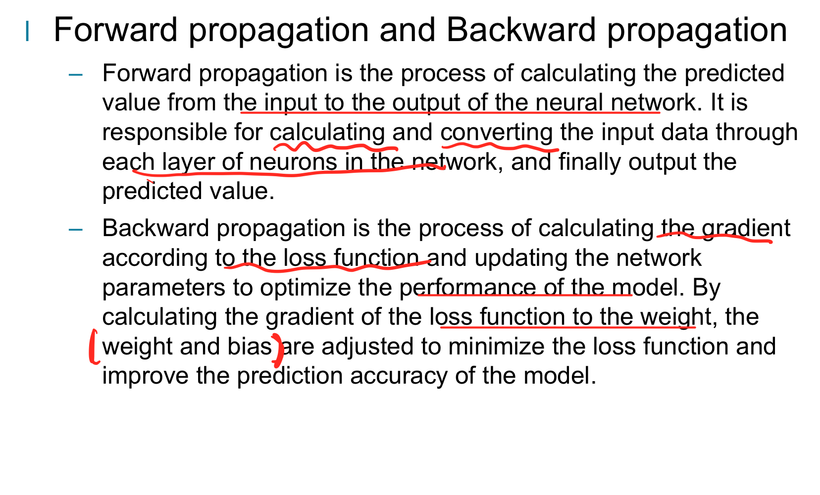
In backpropagation, we start at the output layer, calculate the error terms for each neuron layer by layer (that is, the derivative of the loss function with respect to the activation value of that layer), and then use these error terms and the activation value of the previous layer to calculate the gradient of the weight of the current layer.
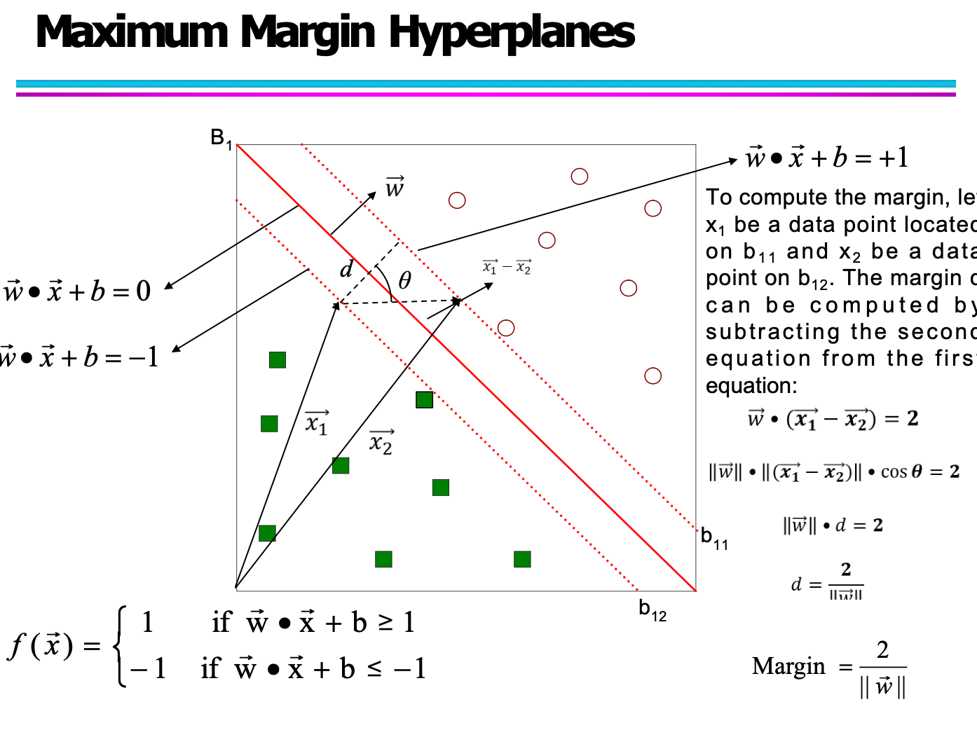
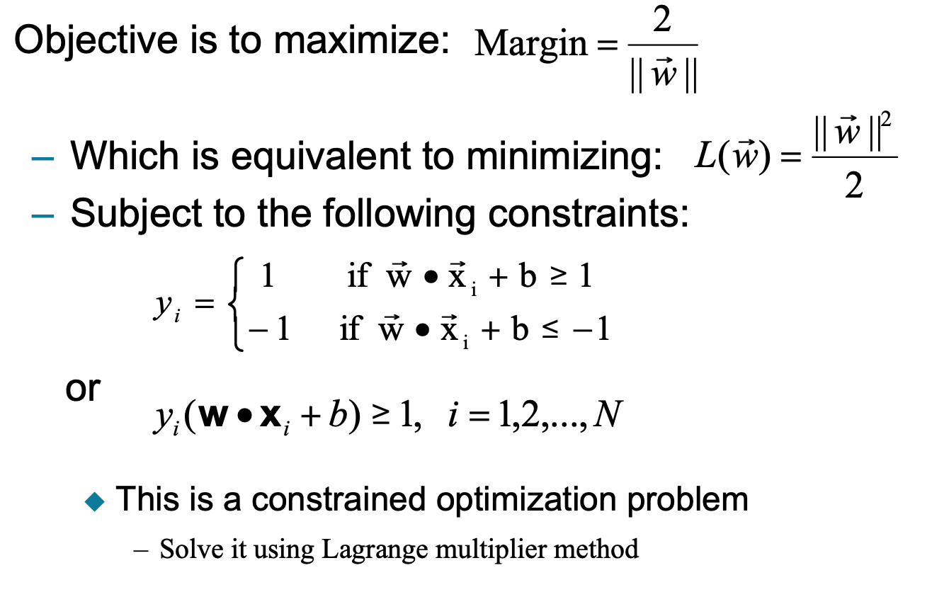
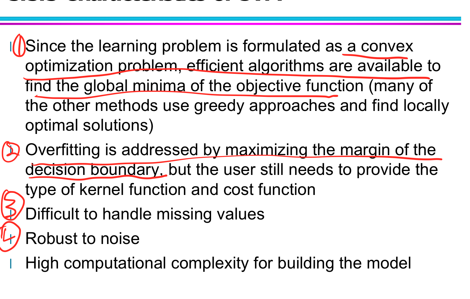
8-3 SVM
Find hyperplane maximizes the margin.
Learning Nonlinear SVM: The Kernel Trick
Support Vector Machines (SVMs) are originally designed for linear classification. To handle nonlinear data, we use the Kernel Trick — a powerful method to implicitly map input data to a higher-dimensional space without actually performing the transformation.
Core Idea: Kernel Trick
Instead of explicitly mapping input x to a high-dimensional space \phi(x), we compute the inner product in that space using a kernel function:
$\phi(x_i) \cdot \phi(x_j) = K(x_i, x_j)$
- $\phi(x)$: Mapping to higher-dimensional space
- $K(x_i, x_j)$: Kernel function, computed in the original space
- No need to compute $\phi(x)$ explicitly!
What Is a Kernel Function?
A kernel function is defined in the original input space and returns the dot product of the corresponding mapped vectors in a high-dimensional feature space.
Common Kernel Functions:
| Kernel Type | Formula | Notes |
|---|---|---|
| Polynomial Kernel | $$K(x, y) = (x \cdot y + 1)^p$$ | |
| Captures polynomial interactions | ||
| Gaussian (RBF) | $$ K(x, y) = e^{- \frac{ | |
| Sigmoid Kernel | $K(x, y) = \tanh(kx \cdot y - \delta)$ | Inspired by neural activation |
Why It Matters
- Avoids expensive computation in high-dimensional space
- Enables SVM to find nonlinear decision boundaries
- Makes SVM extremely flexible for complex datasets:
Kernel Functions: Advantages and Validity Conditions
Advantages of Using Kernel Functions
Kernel functions are central to nonlinear SVMs, allowing computations in high-dimensional spaces without explicitly mapping the data:
- You do not need to know the mapping function φ. The kernel trick computes the inner product in high-dimensional space implicitly.
- Computing φ(xᵢ) • φ(xⱼ) in the original space helps avoid the curse of dimensionality, which occurs when data is explicitly mapped to high-dimensional spaces.
This makes SVMs with kernel functions computationally efficient while still allowing flexible decision boundaries.
Not All Functions Are Valid Kernels
A valid kernel must correspond to an inner product in some feature space. Arbitrary functions may not satisfy the mathematical properties required to be used as kernels.
Support vectors
In Support Vector Machines (SVM), support vectors are the data samples that lie closest to the decision boundary (the separating hyperplane). These are the critical points that directly influence the position and orientation of the hyperplane.
What Are Support Vectors?
-
They are the data points from each class that lie on the margin boundaries.
-
In the canonical form of SVM, they satisfy:
$\vec{w} \cdot \vec{x}_i + b = \pm1$
-
All other data points do not affect the final decision boundary—only the support vectors do.
What Do They Do?
- Define the margin: The distance between the support vectors and the hyperplane is the margin. SVM maximizes this margin.
- Determine the hyperplane: If you remove non-support vectors, the hyperplane stays the same. If you remove support vectors, the hyperplane changes.
- Control generalization: The fewer support vectors used, the better the model may generalize (less overfitting).
Association Analysis
Rules originating from the same itemset have identical support but can have different confidence.
If the itemset is infrequent, then all six candidate rules can be pruned immediately without computing their confidence values.
Association Rule Mining Task
Association rule mining is a key technique in data mining, often used in market basket analysis to discover relationships between items in transactional data. The process is typically divided into two main ste
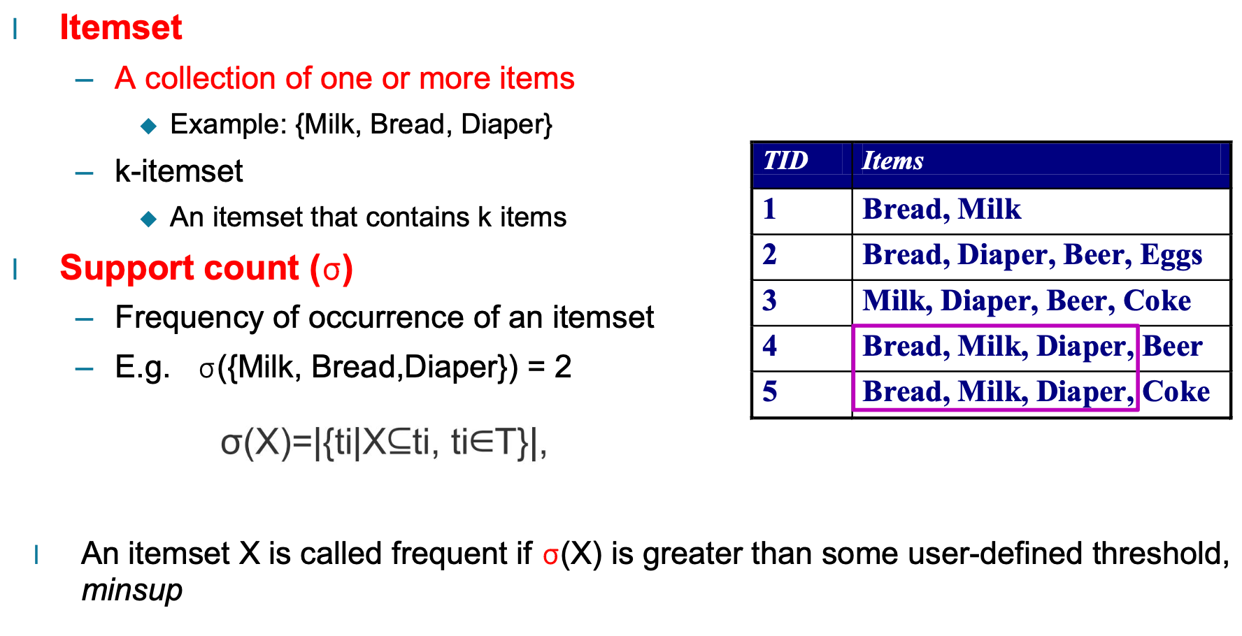
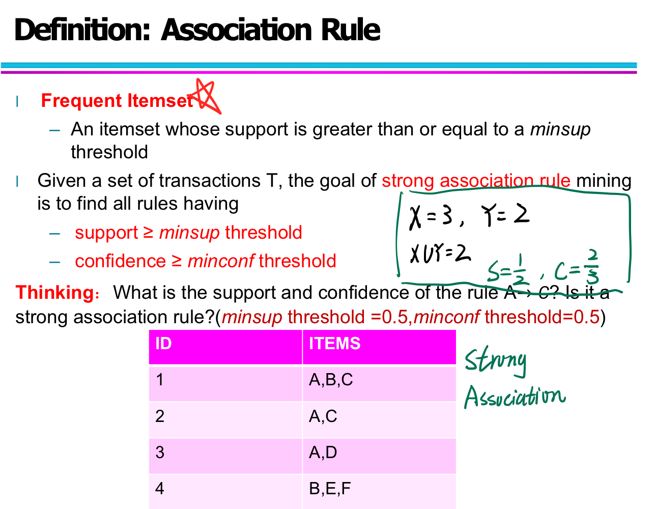
Step 1: Frequent Itemset Generation
- Generate all itemsets that have support ≥ minsup (minimum support threshold).
- These itemsets occur frequently enough in the transaction database to be considered interesting.
- Example: {Milk, Bread} appears in 3 out of 5 transactions → support = 0.6
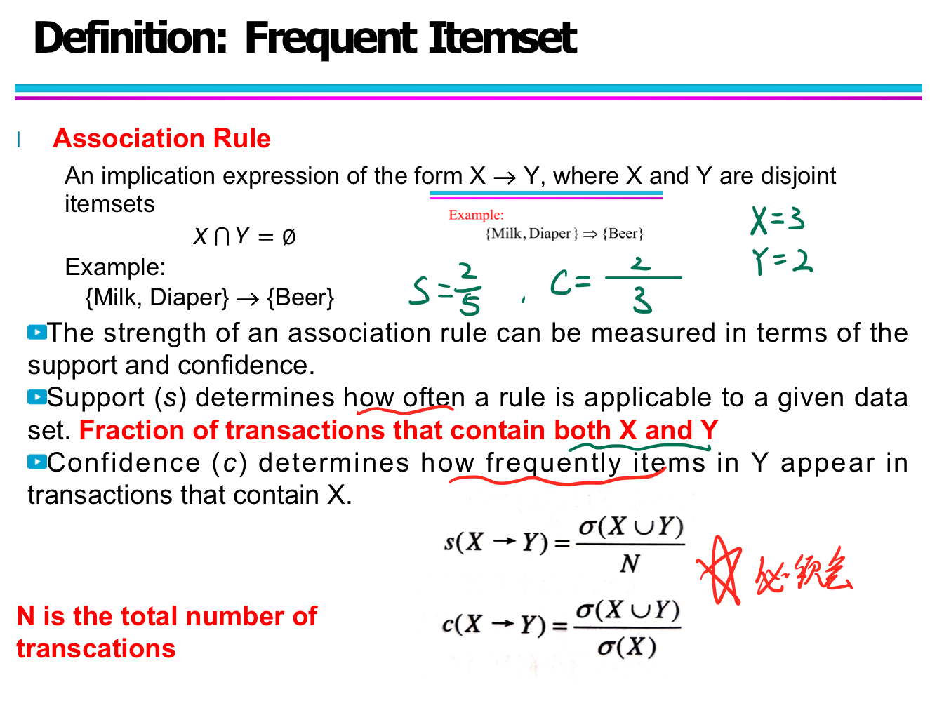
Step 2: Rule Generation
-
From each frequent itemset, generate rules of the form X → Y (where X ∩ Y = ∅).
-
For each rule, calculate confidence:
$\text{confidence}(X \rightarrow Y) = \frac{\sigma(X \cup Y)}{\text{N}(X)}$
-
Retain only rules where confidence ≥ minconf (minimum confidence threshold).
-
These are called strong association rules.
Brute-Force Approach (Inefficient Baseline)
- List all possible association rules from all itemsets.
- Compute the support and confidence for each rule.
- Prune any rules that fail to meet the minsup or minconf thresholds.
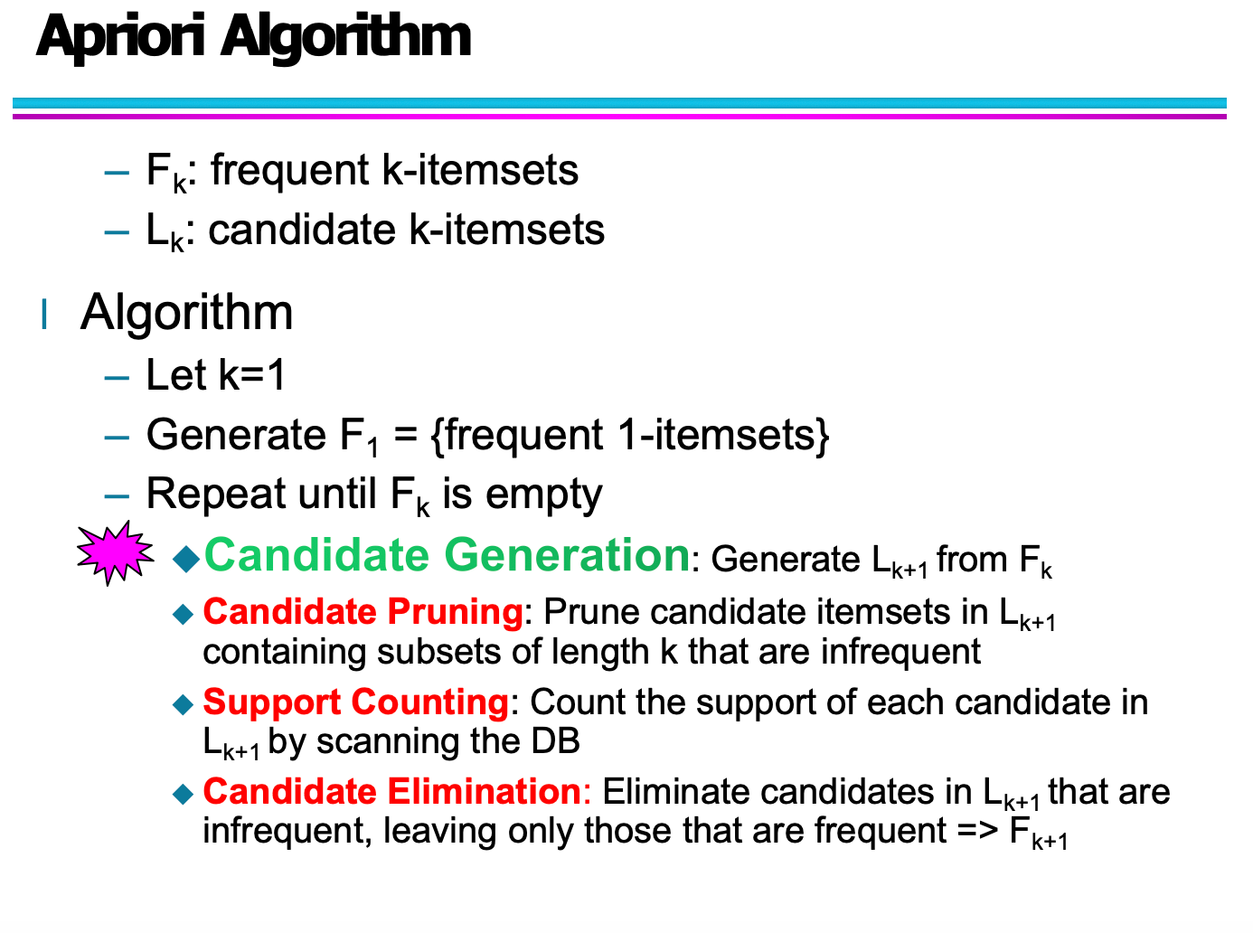
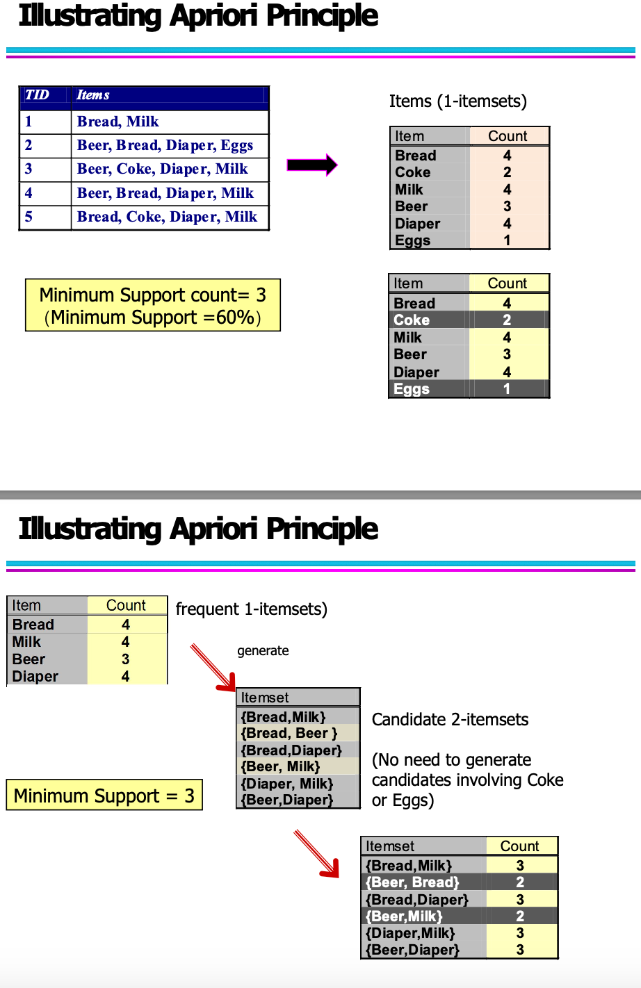
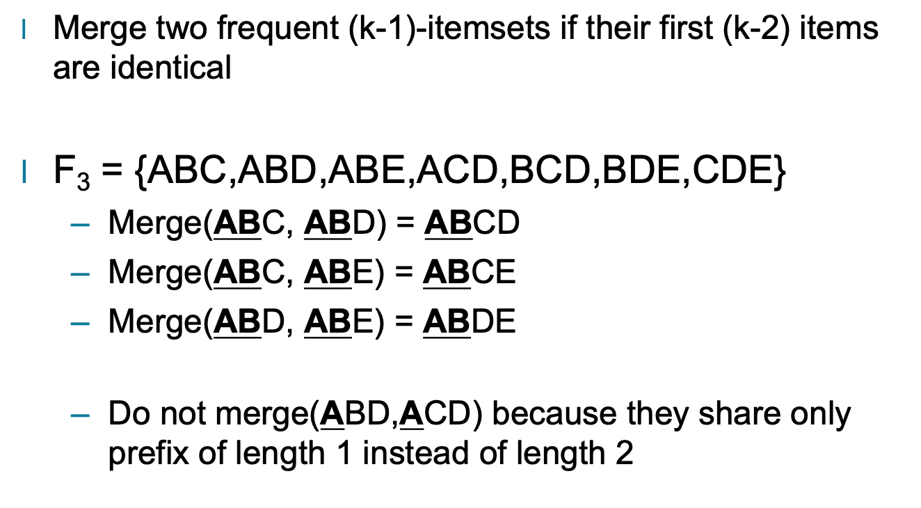
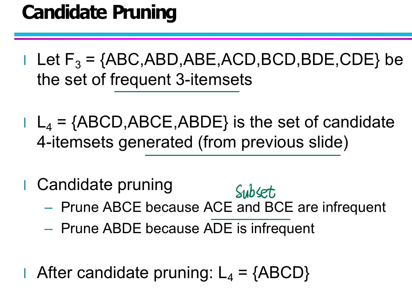
Candidate Generation: Fk-1 x Fk-1 (k≥3)
Before rule generation, confidence is not considered!!
Rule Generation
After frequent item-set generation completed, the support is already guaranteed.

Rule Generation: Confidence and Anti-Monotonicity
When generating association rules from frequent itemsets, confidence is used to measure the strength of a rule. Understanding how confidence behaves with respect to the rule structure is critical for pruning and efficiency.
Confidence Is Not Anti-Monotonic in General
-
In general, confidence does not follow the anti-monotone property with respect to the left-hand side (LHS) of a rule.
-
Example:
$\text{conf}(ABC \rightarrow D) \text{ may be greater or smaller than } \text{conf}(AB \rightarrow D)$
-
Therefore, we cannot prune rules just because a shorter LHS has low confidence.
But Confidence Is Anti-Monotonic Within the Same Frequent Itemset
-
If we fix a frequent itemset L, and generate rules of the form:
$f \rightarrow L - f$
then confidence decreases as the right-hand side (RHS) becomes larger.
-
Example:
-
If $L = {A, B, C, D},$ then:
$\text{conf}(ABC \rightarrow D) \geq \text{conf}(AB \rightarrow CD) \geq \text{conf}(A \rightarrow BCD$)
-
-
This is known as the anti-monotone property of confidence with respect to the size of the RHS.
Why It Matters
- This anti-monotonicity allows efficient pruning during rule generation:
- If a rule with RHS = Y is not strong, then any rule with RHS ⊃ Y can be safely discarded.
- Helps reduce the number of confidence checks needed.
Deep Learnig
Why deep network instead of fat network?
Stronger Expressive Power: Deep networks apply multiple layers of nonlinear transformations, allowing them to model complex and abstract relationships in data that shallow networks cannot easily capture — even if made wider.
Efficiency in Parameter Use: Although a single hidden layer network (fat network) can theoretically approximate any function (Universal Approximation Theorem), it may require an exponentially large number of neurons, making it computationally expensive and inefficient.
Better Generalization: Deep architectures can learn hierarchical features (e.g., edges → shapes → objects), which improves their ability to generalize to new, unseen data. Shallow networks often fail to capture such levels of abstraction.
The slides mention:
“Deep networks achieve lossless transfer of information by implicitly transferring information, reducing human bias and improving generalization.”
Simplified End-to-End Learning: Deep networks can learn directly from raw input data, minimizing the need for manual feature engineering. In contrast, shallow networks often require significant pre-processing or domain-specific feature design.
Scalability with Big Data: Deep models can leverage large datasets more effectively by automatically extracting statistical patterns in the data, whereas shallow networks tend to saturate quickly and underfit complex distributions.
In Summary:
Deep networks outperform fat ones by learning layered feature representations, using parameters more efficiently, generalizing better, and achieving state-of-the-art performance in complex tasks.
NN basic
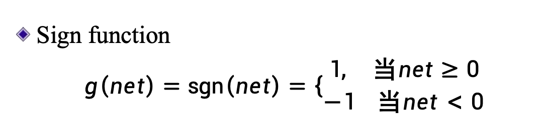
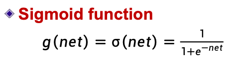
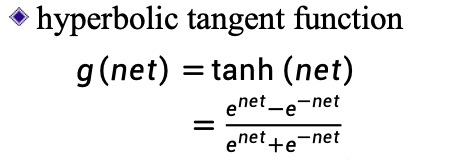
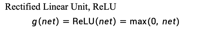
Activation function
CNN
RNN
LLM
🔍 Comparison: One-hot Encoding vs Distributed Representation
| Aspect | One-hot Encoding | Distributed Representation |
|---|---|---|
| Definition | A sparse binary vector with only one dimension set to 1. | A dense, real-valued vector that captures word semantics. |
| Dimensionality | High (equals vocabulary size). | Fixed and low (e.g., 100–300). |
| Semantic Capacity | No semantic information encoded. | Captures similarity between words (e.g., “cat” and “dog” are close). |
| Scalability | Poor – grows with vocabulary size. | Good – constant size regardless of vocabulary. |
| Example | “猫” = [1, 0, 0, 0, 0, 0] | “猫” ≈ [0.2, 0.6, 0.1, 0.7, 0.1] |
| Computation | Simple to create, no training needed. | Requires training (e.g., Word2Vec, GloVe, BERT). |
| Storage Cost | High memory usage. | Low memory footprint. |
| Interpretability | Easy to understand, purely symbolic. | Hard to interpret directly, but powerful. |
| Context Sensitivity | No — static and context-free. | Can be static (Word2Vec) or contextual (e.g., BERT). |
One-hot Encoding
Advantages:
- Simple and intuitive.
- No training required.
Disadvantages:
- Cannot express semantic similarity or meaning.
- Extremely sparse and memory-inefficient.
- Poor performance in most NLP tasks.
Distributed Representation
Advantages:
- Captures rich semantic and syntactic information.
- Compact and computationally efficient.
- Crucial for modern NLP models (e.g., Transformers, BERT).
Disadvantages:
- Requires pretraining or embedding models.
- Less interpretable (vector values don’t have explicit meaning).
- Sensitive to training data quality.